Download
1 / 31
310 likes | 318 Views
Volatility. Chapter 10. Definition of Volatility. Suppose that S i is the value of a variable on day i . The volatility per day is the standard deviation of ln ( S i / S i -1 )

E N D
Volatility Chapter 10
Definition of Volatility • Suppose that Si is the value of a variable on day i. The volatility per day is the standard deviation of ln(Si/Si-1) • Normally days when markets are closed are ignored in volatility calculations (see Business Snapshot 10.1, page 207) • The volatility per year is times the daily volatility • Variance rate is the square of volatility
Implied Volatilities • Of the variables needed to price an option the one that cannot be observed directly is volatility • We can therefore imply volatilities from market prices and vice versa
VIX Index: A Measure of the Implied Volatility of the S&P 500 (Figure 10.1, page 208)
Are Daily Changes in Exchange Rates Normally Distributed? Table 10.1, page 209
Heavy Tails • Daily exchange rate changes are not normally distributed • The distribution has heavier tails than the normal distribution • It is more peaked than the normal distribution • This means that small changes and large changes are more likely than the normal distribution would suggest • Many market variables have this property, known as excess kurtosis
Alternatives to Normal Distributions: The Power Law (See page 211) Prob(v > x) = Kx-a This seems to fit the behavior of the returns on many market variables better than the normal distribution
Standard Approach to Estimating Volatility • Define sn as the volatility per day between day n-1 and day n, as estimated at end of dayn-1 • Define Si as the value of market variable at end of day i • Define ui= ln(Si/Si-1)
Simplifications Usually Made in Risk Management • Defineui as (Si−Si-1)/Si-1 • Assume that the mean value of ui is zero • Replace m-1 by m This gives
Weighting Scheme Instead of assigning equal weights to the observations we can set
ARCH(m) Model In an ARCH(m) model we also assign some weight to the long-run variance rate, VL:
EWMA Model (page 216) • In an exponentially weighted moving average model, the weights assigned to the u2 decline exponentially as we move back through time • This leads to
Attractions of EWMA • Relatively little data needs to be stored • We need only remember the current estimate of the variance rate and the most recent observation on the market variable • Tracks volatility changes • RiskMetrics uses l = 0.94 for daily volatility forecasting
GARCH (1,1), page 218 In GARCH (1,1) we assign some weight to the long-run average variance rate Since weights must sum to 1 g + a + b =1
GARCH (1,1) continued Setting w = gVL the GARCH (1,1) model is and
Example • Suppose • The long-run variance rate is 0.0002 so that the long-run volatility per day is 1.4%
Example continued • Suppose that the current estimate of the volatility is 1.6% per day and the most recent percentage change in the market variable is 1%. • The new variance rate is The new volatility is 1.53% per day
Other Models • Many other GARCH models have been proposed • For example, we can design a GARCH models so that the weight given to ui2 depends on whether uiis positive or negative
Variance Targeting • One way of implementing GARCH(1,1) that increases stability is by using variance targeting • We set the long-run average volatility equal to the sample variance • Only two other parameters then have to be estimated
Maximum Likelihood Methods • In maximum likelihood methods we choose parameters that maximize the likelihood of the observations occurring
Example 1 (page 220) • We observe that a certain event happens one time in ten trials. What is our estimate of the proportion of the time, p, that it happens? • The probability of the outcome is • We maximize this to obtain a maximum likelihood estimate: p = 0.1
Example 2 (page 220-221) Estimate the variance of observations from a normal distribution with mean zero
Application to GARCH (1,1) We choose parameters that maximize
Calculations for Yen Exchange Rate Data (Table 10.4, page 222)
Forecasting Future Volatility (Equation 10.14, page 226) A few lines of algebra shows that To estimate the volatility for an option lasting T days we must integrate this from 0 to T
Forecasting Future Volatility cont The volatility per year for an option lasting T days is
Volatility Term Structures (Equation 10.16, page 228) • The GARCH (1,1) model allows us to predict volatility term structures changes • When s(0) changes by Ds(0), GARCH (1,1) predicts that s(T) changes by