Download

1 / 26
260 likes | 384 Views
Volatility. Downloads. Today’s work is in: matlab_lec04.m Functions we need today: simsec.m, simsecJ.m, simsecSV.m Datasets we need today: data_msft.m. Homework 1. function r=simsec(mu,sigma,T); x=randn(T,1); for t=1:T; r(t,1)=exp(mu+sigma*x(t))-1; end;.

E N D
Downloads • Today’s work is in: matlab_lec04.m • Functions we need today: simsec.m, simsecJ.m, simsecSV.m • Datasets we need today: data_msft.m
Homework 1 function r=simsec(mu,sigma,T); x=randn(T,1); for t=1:T; r(t,1)=exp(mu+sigma*x(t))-1; end;
Simulate Simple Process >>data_msft; >>subplot(2,1,1); hist(msft(:,4),[-.2:.01:.2]); >>sigma=std(msft(:,4)); >>mu=mean(msft(:,4))-.5*sigma^2; T=length(msft); >>r=simsec(mu,sigma,T); >>disp([mean(msft(:,4)) mean(r)]); >>disp([std(msft(:,4)) std(r)]); >>disp([skewness(msft(:,4)) skewness(r)]); >>disp([kurtosis(msft(:,4)) kurtosis(r)]); >>subplot(2,1,2); hist(r,[-.2:.01:.2]);
Compare simulated to actual • Mean, standard deviation, skewness match well • Kurtosis (extreme events) does not match well • Actual has much more mass in the tails (fat tails) • This is extremely important for option pricing! • CLT fails when tails are “too” fat
ModellingVolatility • How to make tales fatter? • Add jumps to log normal distribution to make tails fatter • Jumps also help with modeling default • Make volatility predictable: • Stochastic volatility, governed by state variable • ARCH process (2003 Nobel prize, Rob Engle)
Jumps • R(t)=exp(µ+σ*X(t)+J(t)) • J(t)=J1 with p1, J2 with p2, 0 with 1-p1-p2 >>nlow=sum(msft(:,4)<-.1); >>nhigh=sum(msft(:,4)>.1); >>[T a]=size(msft); >>p1=nlow/T; p2=nhigh/T; >>J1=-.15; J2=.15;
Simulating Jumps function r=simsecJ(mu,sigma,J1,J2,p1,p2,T); x=randn(T,1); y=rand(T,1); for t=1:T; if y(t)<p1; J(t)=J1; elseif y(t)<p1+p2; J(t)=J2; else J(t)=0; end; r(t)=exp(mu+sigma*x(t)+J(t))-1; end;
Simulating Jumps >>r=simsecJ(mu,sigma,J1,J2,p1,p2,T); >>disp([mean(msft(:,4)) mean(r)]); >>disp([std(msft(:,4)) std(r)]); >>disp([skewness(msft(:,4)) skewness(r)]); >>disp([kurtosis(msft(:,4)) kurtosis(r)]); >>subplot(2,1,2); hist(r,[-.2:.01:.2]); %Note that kurtosis of simulated now matches actual
Stochastic Volatility • Suppose volatility was not constant, but changed through time and was predictable • This is very realistic, volatility tends to be much higher during recessions than expansions; high volatility tends to predict high volatility • That is sigma is replaced by sigma(t)=f(Z(t)) where Z(t) is a random variable
Moving Average • When we have a long time series of data we can calculate the local average a few points around each point in time, this is called a moving average • We will write code to calculate a moving average and use it to analyze stochastic volatility (to be used later as well)
Moving Average >>T1=floor(T/7); ma=zeros(T1,2); >>for i=1:T1; in=(i-1)*7+1:(i-1)*7+7; ma(i,1)=std(msft(in,4)); ma(i,2)=mean(msft(in,4).^2); for j=1:7; t=(i-1)*7+j; ma(i,2)=ma(i,2)+(msft(t,4)^2)/7; end; end; >>disp(corrcoef(ma(:,1),ma(:,2)));
>>subplot(3,1,1); plot(ma(:,1)); >>subplot(3,1,2); plot(ma(:,2)); >>WN=exp(randn(T1,1)); subplot(3,1,3); plot(WN);
regress() • regcoef=regress(Y,X) regresses vector time series Y on multiple time series in X • regcoef contains the regression coefficients • Y must be Tx1, X must be TxN where N is the number of regressors • If you want a constant in your regression, first column of X must be all 1’s • ie y(t)=A+B*x(t), than Y=[y(1); y(2); … y(T)], X=[1 x(1); 1 x(2); … 1 x(T)] • [a1 a2]=regress(Y,X) gives coefficients in a1, and 95% bounds in a2 • [a1 a2 a3 a4 a5]=regress(Y,X) gives coefficients in a1, 95% bounds in a2, R2 in a5(1)
No predictability in WN >>X=[ones(T1-1,1) WN(1:T1-1,1)]; >>Y=WN(2:T1,1); >>[regcoef sterr a3 a4 rsq]=regress(Y,X); >>disp([regcoef sterr]); • Note regcoef(2) is close to zero and sterr(2,:) is not significant disp(rsq(1)); • Note, R2 is close to zero
Predictability in Volatility >>X=[ones(T1-1,1) ma(1:T1-1,2)]; >>Y=ma(2:T1,2); >>[regcoef sterr a3 a4 rsq]=regress(Y,X); >>disp([regcoef sterr]); %Note regcoef(2) is positive and significant! >>disp(rsq(1)); %Note, R2 is 14.86%! %Even with a simple linear model we get %predictability! Can you think of better models?
Scatter Plot >>subplot(2,1,1); plot(WN(1:T1-1,1),WN(2:T1,1),'.'); >>subplot(2,1,2); plot(ma(1:T1-1,2),ma(2:T1,2),'.');
Discrete, Markov volatility • sigma(t)=.015 or .025 (daily) • When sigma(t)=.015, it will be .015 with probability .9 tomorrow, and will be .025 with probability .1 tomorrow • When sigma(t)=.025, it will be .025 with probability .9 tomorrow, and will be .015 with probability .1 tomorrow • Transition probability matrix: [.9 .1; .1 .9] • This is a 2-state Markov process, it is predictable, when sigma(t) is high, it is likely to stay high
AR(1) Volatility • Let Z(t) be a normal rv • Let W(t)=ρSW(t-1)+σSZ(t) • This is called an AR(1) process, as you can see it is predictable, W(t) is expected to be high when W(t-1) is high • Let σ(t)=µS+W(t) • Do you see any problems with this process? • If σS=0 than σ(t)=µS so constant vol • If ρS=0 than σ(t) is i.i.d. and there is no persistence in vol
Simulating Stochastic Vol function r=simsecSV(mu,muS,J1,J2,p1,p2,rho,sigmaS,T); x=randn(T,1); y=rand(T,1); z=randn(T+1,1); W(1)=0; J=zeros(T,1); r=zeros(T,1); for t=1:T; W(t+1)=rho*W(t)+sigmaS*z(t+1); sigma(t)=abs(muS+W(t)); if y(t)<p1; J(t)=J1; elseif y(t)<p1+p2; J(t)=J2; else J(t)=0; end; r(t)=exp(mu+sigma(t)*x(t)+J(t))-1; end;
Moving Averageof Simulated sigmaS=.0025; rho=.96; r=simsecSV(mu,sigma,J1,J2,p1,p2,rho,sigmaS,T); T1=floor(T/7); masim=zeros(T1,2); for i=1:T1; in=(i-1)*7+1:(i-1)*7+7; masim(i,1)=std(r(in,1)); masim(i,2)=mean(r(in,1).^2); for j=1:7; t=(i-1)*7+j; masim(i,2)=masim(i,2)+(r(t,1)^2)/7; end; end;
>>X=[ones(T1-1,1) masim(1:T1-1,1)]; Y=masim(2:T1,1); >>[regcoef sterr a3 a4 rsq]=regress(Y,X); >>disp([regcoef sterr]); disp(rsq(1)); >>subplot(2,1,1); plot(ma(:,1)) >>subplot(2,1,2); plot(masim(:,1));
OptionalHomework (2) • Use the function from Homework (1) to simulate Microsoft daily returns for a period of a year many times, over and over again • Each time record the total return for the year • This is called Monte-Carlo simulation • How likely is it that Microsoft loses 30% in one year? How likely is it to lose 40%? • Separate the worst 5% of years from the next 95%. What is the value lost at the 5% break? This is called Value at Risk, it is a commonly used risk measure • How sensitive is Value at Risk to jump parameters? Jump events are quite rare, do you think they are easy to estimate?
OptionalHomework (3) • Extend the model by adding stochastic volatility, try both the discrete Markov and the AR(1) process (AR(1) case done in class in file simsecSV.m) • How does this change kurtosis and likelyhood of tail events? • Plot a time series of squared Microsoft returns and squared simulated returns (with and without stochastic volatility) • Does it look like high times are followed by high times in the data? In the model with no stochastic vol? In the model with stochastic vol? • Do you see any problems with the AR(1) formulation for volatility? • Does Value at Risk change during high volatility and low volatility times?