Keary & Brooks – Chapter 5

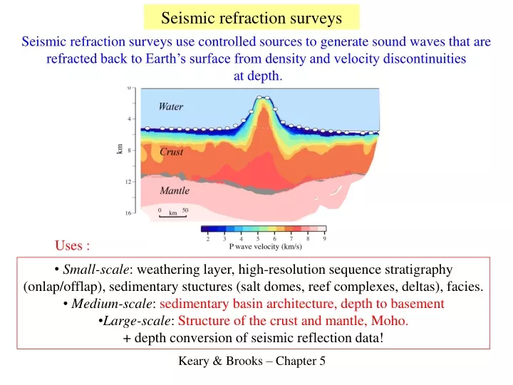
1. Seismic refraction surveys Seismic refraction surveys use controlled sources to generate sound waves that are refracted back to Earth’s surface from density and velocity discontinuities at depth. Uses : • Small-scale: weathering layer, high-resolution sequence stratigraphy (onlap/offlap), sedimentary stuctures (salt domes, reef complexes, deltas), facies. • Medium-scale: sedimentary basin architecture, depth to basement • Large-scale: Structure of the crust and mantle, Moho. • + depth conversion of seismic reflection data! Keary & Brooks – Chapter 5

2. Two horizontal layers This is the travel time of the refracted wave. The refracted wave propagates along a buried interface at the velocity of the lower medium. They are normally the first phases to arrive at a receiver and hence are called head waves.

3. Time-Distance Plot At the the cross-over distance, xcros, travel times of the direct and refracted arrivals are equal. T The thickness of the upper of the two layers, z, can be determined from the cross-over distance and the velocities or the intercept time and the velocities.

4. Direct, reflected and head wave fronts Geophone number Elapsed time after shot (s) Offset (m) Depth (m)

5. Multiple layers Head wave Head wave Direct wave ABCDEF is the refracted ray path through the bottom layer of a three layer model. The travel time curve for the direct and two head waves are shown above.

6. The velocity V3 can be estimated from the slope of the second head wave. V1 and V2 can be estimated from the direct and first head wave and z1 and z2 from the intercept times This gives the travel time, Tn of a ray critically refracted along the top surface of the n th horizontal layer

7. Mendips field data V2=1.89 km/s V3=5.84 km/s

8. Common shot point gathers from 3 streamers (6,15,6 km) 3.1 km/s 1.5 km/s

9. Seismic refraction using Ocean Bottom Seismometers (OBSs) 4-channel: hydrophone + 3 component seismometer Data logger + batteries + GPS clock Ballast weights (for coupling with seabed) Hydro-acoustic release Titanium tubes for > 6000 m Operation: 10-360 days

10. OBS DataReduced time Vs. distance plots (A 6m/s refractor will appear flat)

11. Dipping layers Shoot down-dip Shoot up-dip

12. Down-dip: Up-dip: θ and γ can be estimated from the velocities V1, V2u and V2d and hence z and z’ and h and h’ calculated. See Keary & Brooks (Chap 5) + Practical 4

13. Offsets in the travel time Vs. distance plot for head waves from opposite sides of a fault Δt The throw on the fault, Δz, can be calculated from the travel time offset, Δt Note: Valid only for small throws cf. refractor depth.

14. Thin and low velocity layers A thin layer that does not generate a head wave that is a first arrival A low velocity layer that does not generate a head wave

15. Non-planar refractor geometry Reference (dashed lines) show the planar case M (e.g.) is nearer the surface than the reference interface, the actual travel time to M’ plots below the reference line. Conversely, that for N’ is above it. These observations can be quantified using the concept of delay time.

16. The concept of delay time We can think of the travel time of a refracted wave being made up of 3 parts: the time it takes to travel between the source and receiver, SvRv, at velocity V2, plus a term at the source, δS, to equal the time it takes to go from S to C at velocity V1, and an equivalent term, δR, at the receiver. where δS and δR are called the delay times

17. Determining lateral variations in layer thickness The time, tf, to go from one end to a receiver (SfCDR),and then on to the other end,tr, (REFSr), is longer than the total time, ttotal, to go from end to end (SfCDEFSr), because of the extra times to travel from the interface to the receiver, along DR and ER. hR tf, tr and ttotal can be read off from a travel time Vs. distance plot and the delay time calculated. The depth to the interface at R can then be calculated from the delay time and the velocities.

18. Generalized velocity structure of continental and oceanic crust

19. Velocity Vs. depth Moho White et al. (1992) Velocities increase gradually through the oceanic crust (difficult to fit straight lines on Time Vs. distance plots). Moho is usually marked by a velocity jump to > 8.0 km/s

20. Amazon margin, NE Brazil: Line B - CDP Stack Fan channel-levee system Late Miocene - Pleistocene Late Albian - Mid-Miocene Oceanic crust SW NE Seafloor multiple Reflectors showing aggradation and fan deposition OBS 315 Moho??

21. Line B: Refraction and velocity model Iso-velocity contours showing progradation and facies Moho

22. OBS surveys and the Continental/Ocean Transition (COT) at conjugate rifted margins