Download

1 / 52
520 likes | 625 Views
Introduction to M ATLAB Programming. Ian Brooks Institute for Climate & Atmospheric Science School of Earth & Environment i.brooks@see.leeds.ac.uk. Course Resources. Course web page: http ://homepages.see.leeds.ac.uk/~ lecimb/matlab/index.html Course power point slides Exercises .

E N D
Introduction to MATLAB Programming Ian BrooksInstitute for Climate & Atmospheric ScienceSchool of Earth & Environment i.brooks@see.leeds.ac.uk
Course Resources Course web page: • http://homepages.see.leeds.ac.uk/~lecimb/matlab/index.html • Course power point slides • Exercises
What is MATLAB? • Data processing and visualization tools • Easy, fast manipulation and processing of complex data • Visualization to aid data interpretation • Production of publication quality figures • High-level programming languages • Can write extensive programs, applications,… • Faster code development than with C, Fortran, etc. • Possible to “play” with or “explore” data – don’t have to write a standalone program to do a predetermined job
Getting started – linux (SEE) Just enter ‘matlab’ or ‘matlab &’ on the command line Might need to run ‘app setup matlab’ or add this to your .cshrcfile
MATLAB User Environment Workspace/Variable Inspector Command Window Command History
Getting help There are several ways of getting help: Basic help on named commands/functions is echoed to the command window by: >> help command-name A complete help system containing full text of manuals is started by: >> helpdesk
Contents Search Index Demos Help Browser • Contents - browse through topics in an expandable "tree view" • Index - find topics using keywords • Search - search the documentation. There are four search types available: • Full Text - perform a full-text search of the documentation • Document Titles - search for word(s) in documentation section titles • Function Name - see reference descriptions of functions • Online Knowledge Base - search the Technical Support Knowledge • Base • Demos – view and run product demos
Other sources of help • www.mathworks.com • Help forums, archived questions & answers, archive of user-submitted code • http://lists.leeds.ac.uk/mailman/listinfo/see-matlab • Mailing list for School of Earth & Environmentself-help from other users within the school (31 at last count)
Array Editor For editing 2-D numeric arrays double-click
Calculations on the command Line MATLAB as a calculator Assigning Variables • >> -5/(4.8+5.32)^2 • ans = • -0.048821 • >> (3+4i)*(3-4i) • ans = • 25 • >> cos(pi/2) • ans = • 6.1232e-017 • >> exp(acos(0.3)) • ans = • 3.547 >> a = 2; >> A = 5; >> a^A ans = 32 >> x = 5/2*pi; >> y = sin(x) y = 1 >> z = asin(y) z = 1.5708 Semicolon suppresses screen output Variables are case sensitive Results assigned to “ans” if name not given Use parentheses ( ) for function inputs Numbers stored in double-precision floating point format
The WORKSPACE • MATLAB maintains an active workspace, any variables (data) loaded or defined here are always available. • Some commands to examine workspace, move around, etc: who: lists the variables defined in workspace >> who Your variables are: x y
whos: lists names and basic properties of variables in the workspace >> whos Name Size Bytes Class x 3x1 24 double array y 3x2 48 double array Grand total is 9 elements using 72 bytes
Entering Numeric Arrays Row separator: Semicolon (;) or newline Column separator: space or comma (,) >> a=[1 2;3 4] a = 1 2 3 4 >> b = [2:-0.5:0] b = 2 1.5 1 0.5 0 >> c = rand(2,4) c = 0.9501 0.6068 0.8913 0.4565 0.2311 0.4860 0.7621 0.0185 Use square brackets [ ] Creating sequences using the colon operator (:) Utility function for creating matrices. Matrices must be rectangular. (Undefined elements set to zero)
Entering Numeric Arrays (Continued) Using other MATLAB expressions >> w = [-2.8, sqrt(-7), (3+5+6)*3/4] w = -2.8 0 + 2.6458i 10.5 >> m(3,2) = 3.5 m = 0 0 0 0 0 3.5 >> w(2,5) = 23 w = -2.8 0 + 2.6458i 10.5 0 0 0 0 0 0 23 Matrix element assignment Adding to an existing array Note: MATLAB deals with Imaginary numbers…
Columns (n) 1 2 3 4 5 A = 1 6 11 16 21 2 7 12 17 22 3 8 13 18 23 4 9 14 19 24 5 10 15 20 25 4 10 1 6 2 A (2,4) 1 2 Rows (m) 3 4 5 8 1.2 9 4 25 7.2 5 7 1 11 A (17) 0 0.5 4 5 56 23 83 13 0 10 Indexing into a Matrix in MATLAB Rectangular Matrix: Scalar: 1-by-1 array Vector: m-by-1 array 1-by-n array Matrix: m-by-n array
Array Subscripting / Indexing 1 2 3 4 5 A = 1 6 11 16 21 2 7 12 17 22 3 8 13 18 23 4 9 14 19 24 5 10 15 20 25 4 10 1 6 2 1 2 3 4 5 8 1.2 9 4 25 A(1:5,5) A(:,5) A(21:25) A(1:end,end) A(:,end) A(21:end)’ 7.2 5 7 1 11 0 0.5 4 5 56 A(3,1) A(3) 23 83 13 0 10 A(4:5,2:3) A([9 14;10 15]) • Use () parentheses to specify index • colon operator (:) specifies range / ALL • [ ] to create matrix of index subscripts • 'end' specifies maximum index value
THE COLON OPERATOR • Colon operator occurs in several forms • To indicate a range (as above) • To indicate a range with non-unit increment >> N = 5:10:35 N = 5 15 25 35 >> P = [1:3; 30:-10:10] P = 1 2 3 30 20 10
To extract ALL the elements of an array (extracts everything to a single column vector) >> A = [1:3; 10:10:30; 100:100:300] A = 1 2 3 10 20 30 100 200 300 >> A(:) ans = 1 10 100 2 20 200 3 30 300
Numerical Array Concatenation [ ] Use [ ] to combine existing arrays as matrix “elements” >> a=[1 2;3 4] a = 1 2 3 4 >> cat_a=[a, 2*a; 3*a, 4*a; 5*a, 6*a] cat_a = 1 2 2 4 3 4 6 8 3 6 4 8 9 12 12 16 5 10 6 12 15 20 18 24 Use square brackets [ ] Row separator: semicolon (;) Column separator: space / comma (,) 4*a N.B. Matrices MUST be rectangular.
Matrix Operators Array operators parentheses () complex conjugate transpose array transpose ' .' power array power ^ .^ multiplication array mult. * .* division array division / ./ left division \ addition + subtraction - Matrix and Array Operators Common Matrix Functions inv matrix inverse det determinant rank matrix rank eig eigenvectors and eigenvalues svd singular value dec. norm matrix / vector norm >> help matfun >> help ops
1 & 2D arrays are treated as formal matrices • Matrix algebra works by default: 1x2 row oriented array (vector)(Trailing semicolon suppresses display of output) >> a=[1 2]; >> b=[3 4]; >> a*b ans = 11 >> b*a ans = 3 6 4 8 2x1 column oriented array Result of matrix multiplication depends on order of terms (non-cummutative)
Element-by-element (array) operation is forced by preceding operator with a period ‘.’ >> a=[1 2]; >> b=[3 4]; >> c=[3 4]; >> a.*b ??? Error using ==> times Matrix dimensions must agree. >> a.*c ans = 3 8 Size and shape must match
>> w=[1 2;3 4] + 5 1 2 = + 5 3 4 1 2 5 5 = + 3 4 5 5 6 7 = 8 9 Matrix Calculation-Scalar Expansion >> w=[1 2;3 4] + 5 w = 6 7 8 9 Scalar expansion
>> a = [1 2 3;4 5 6]; >> b = [3,1;2,4;-1,2]; >> c = a*b c = 4 15 16 36 [2x3] [3x2] [2x3]*[3x2] [2x2] a(2nd row).b(2nd column) Matrix Multiplication • Inner dimensions must be equal. • Dimension of resulting matrix = outermost dimensions of multiplied matrices. • Resulting elements = dot product of the rows of the 1st matrix with the columns of the 2nd matrix.
Array (element-by-element) Multiplication • Matrices must have the same dimensions (size and shape) • Dimensions of resulting matrix = dimensions of multiplied matrices • Resulting elements = product of corresponding elements from the original matrices • Same rules apply for other array operations >> a = [1 2 3 4; 5 6 7 8]; >> b = [1:4; 1:4]; >> c = a.*b c = 1 4 9 16 5 12 21 32 c(2,4) = a(2,4)*b(2,4)
>> a=[1 2] A = 1 2 >> b=[3 4]; >> a.*b ans = 3 8 >> c=a+b c = 4 6 No trailing semicolon, immediate display of result Element-by-element multiplication Matrix addition & subtraction operate element-by-element anyway. Dimensions of matrix must still match!
>> A = [1:3;4:6;7:9] A = 1 2 3 4 5 6 7 8 9 >> mean(A) ans = 4 5 6 >> sum(A) ans = 12 15 18 >> mean(A(:)) ans = 5 Many common functions operate on columns by default Mean of each column in A Mean of all elements in A
Clearing up >> clearclear all workspace >> clear VARNAME clear named variable >> clear all clear everything (see help clear) >> close all close all figures >> clc clears command window display only
Boolean (logical) operators isempty() true if matrix is empty, [] isfinite() true where elements are finite isinf() true where elements are infinite any() true if any element is non-zero all() true is all elements are non-zero zeros([m,n]) - create an m-by-n matrix of zeros zeros(size(A)) - create a matrix of zeros the same size as A == is equal to > greater than < less than >= greater than or equal to <= less than or equal to ~ not & and | or
LOGICAL INDEXING • Instead of indexing arrays directly, a logical mask can be used – an array of same size, but consisting of 1s and 0s (true and false) – usually derived as result of a logical expression. >> X = [1:10] X = 1 2 3 4 5 6 7 8 9 10 >> ii = X>6 ii = 0 0 0 0 0 0 1 1 1 1 >> X(ii) ans = 7 8 9 10
Logical indexing is a very powerful tool for selecting subsets of data. Combine multiple conditions using boolean operators.
>> >> x = [1:10]; >> y = x.^0.5; >> i1 = x >= 5 I1 = 0 0 0 0 1 1 1 1 1 1 >> i2 = y<3 i2 = 1 1 1 1 1 1 1 1 0 0 >> ii = i1 & i2 ii = 0 0 0 0 1 1 1 1 0 0 >> find(ii) ans = 5 6 7 8 Find function converts logical index to numeric index
>> plot(x,y,’bo’) >> plot(x(ii),y(ii),’ro’)
Basic Plotting Commands • figure : creates a new figure window • plot(x) : plots line graph of x vs index number of array • plot(x,y) : plots line graph of x vs y • plot(x,y,'r--') : plots x vs y with linetype specified in string : 'r' = red, 'g'=green, etc for a limited set of basic colours. '' solid line, ' ' dashed, 'o' circles…see graphics section of helpdesk