Download
1 / 20
210 likes | 366 Views
Smith Chart. Impedance measured at a point along a transmission line depends not only on what is connected to the line , but also on the properties of the line , and where the measurement is made physically, along the transmission line, with respect to the load (possibly an antenna).

E N D
Smith Chart Impedance measured at a point along a transmission line depends not only on what is connected to the line, but also on the properties of the line, and where the measurement is made physically, along the transmission line, with respect to the load (possibly an antenna).
Smith Chart The SMITH chart is a graphical calculator that allows the relatively complicated mathematical calculations, which use complex algebra and numbers, to be replaced with geometrical constructs, and it allows us to see at a glance what the effects of altering the transmission line (feed) geometry will be. If used regularly, it gives the practitioner a really good feel for the behaviour of transmission lines and the wide range of impedance that a transmitter may see for situations of moderately high mismatch (VSWR).
Smith Chart The SMITH chart lets us relate the complex dimensionless number gamma at any point P along the line, to the normalised load impedance zL = ZL/Zo which causes the reflection, and also to the distance we are from the load in terms of the wavelength of waves on the line
Smith Chart Traveling Waves
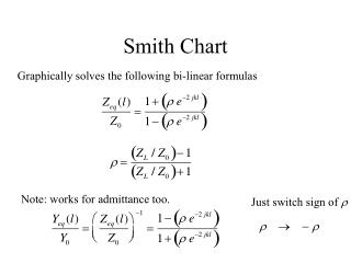
Smith Chart It is a polar plot of the complex reflection coefficient (called gamma herein), or also known as the 1-port scattering parameter s or s11, for reflections from a normalised complex load impedance z = r + jx; the normalised impedance is a complex dimensionless quantity obtained by dividing the actual load impedance ZL in ohms by the characteristic impedance Zo (also in ohms, and a real quantity for a lossless line) of the transmission line.
Smith Chart How it works = (ZR – Z0) / (ZR + Z0) For Open circuited line, ZR = , Hence • = (1-Z0/ZR) / (1+ZR/Z0)=1 For Short circuited line, ZR=0, Hence = -Z0/Z0 = -1
Smith Chart How it works Vmax= A + B = A(1+B/A) Vmin=A – B = A(1- B/A) Standing Wave Ratio= Vmax to Vmin s = Vmax / Vmin= (1+B/A)/(1-B/A) Reflection Factor = =B/A 1+ s -1 = S = s +1 1- ZR –Z0 Since = ZR +Z0
Smith Chart 1+ s -1 S = = 1- s +1 S= S=3 = 1 =0.5 0, 1,0
Smith Chart How it works The Smith chart resides in the complex plane of reflection coefficient G = Gr + Gi = | G |ejq = | G |/u. At point A, G = 0.6 + j0.3 = 0.67/26.6°.
Smith Chart How it works Points of constant resistance form circles on the complex reflection-coefficient plane. Shown here are the circles for various values of load resistance.
Smith Chart Values of constant imaginary load impedances xL make up circles centered at points along the blue vertical line. The segments lying in the top half of the complex-impedance plane represent inductive reactances; those lying in the bottom half represent capacitive reactances. Only the circle segments within the green circle have meaning for the Smith chart
Smith Chart How it works The circles (green) of and the segments (red) of lying within the | G | = 1 circle combine to form the Smith chart, which lies within the complex reflection-coefficient (G) plane, shown in rectangular form by the gray grid.
Smith Chart How it works With a Smith chart, you can plot impedance values using the red and green circles and circle segments and then read reflection-coefficient values from the gray grid. Many Smith charts include a scale (yellow) around their circumference that lets you read angle of reflection coefficient.
Smith Chart How it works Standing waves, which repeat for every half wavelength of the source voltage, arise when (b) a matched generator and transmission line drive an unmatched load. (c) Time-varying sine waves of different peak magnitudes appear at different distances along the transmission line as a function of wavelength.
Smith Chart point L represents a normalized load impedance zL = 2.5 – j1 = 0.5/18°.If point L corresponds to | G | = 0.5 and SWR = 3, then any point in the complex reflection-coefficient plane equidistant from the origin must also correspond to | G | = 0.5 and SWR = 3, and a circle centered at the origin and whose radius is the length of line segment OL represents a locus of constant-SWR points. How it works
Smith Chart How it is drawn Normalized Impedances: R+JL=R+jX Normalized Resistance; r=R/Z0 Normalized Reactance; x=X/Z0 Normalized Impedance; z=Z/Z0=r+jx Normalized Conductance; y=g+jb • Resistance Circles on Horizontal lines are at centre {r/(r+1),0} with radius of 1/(r+1) • Reactance Circles on Vertical lines are at centre {1, 1/x} with radius of 1/x
Smith Chart Problem: 1 Load Impedance ZR= 50 +j100 on a 50 line. Solution:- • Normalize the Impedance; z = 1 +j2.0 • On horizontal Resistance line move from zero to 1.0 on the right • Follow resistance circle upward(+ve immag) • Locate point where crosses reactance circle j2.0 • Point of intersection is z = 1.0 + j2.0
Smith Chart Problem:-Voltage Standing Wave Ratio: ZR=100 – j50 on a 50 line. Find VSWR? Solution: • Normalize Z…zR= 2 – j1.0 • Plot it on the chart • Draw a circle with center at point (1,0)through point zR • VSWR is 2.6
Smith Chart Problem: Reflection Coefficient:- ZR= 100 + j75 on a 50 line Find ? Solution: • Normalize Load zR= 2 + j1.5 • Plot the zR on the chart • Draw VSWR circle through zR, read VSWR…= 3.3 • = (s -1)/(s + 1) ? • = 0.535 • Draw a radial line through zR to meet the phase line…. = 0.535300
Smith Chart Problem: Admittance ZR=150 + j75 on 50 line Find YR? Solution: • Normalize zR; • plot zR; • draw VSWR through zR from the center • Point of intersection yR= 0.27 + 0.14 • Admittance = YR= yR/50 = 0.0054 + j0.0028S