Download
1 / 21
270 likes | 932 Views
Smith Chart. Supplemental Information Fields and Waves I ECSE 2100. Smith Chart. Impedances, voltages, currents, etc. all repeat every half wavelength

E N D
Smith Chart Supplemental Information Fields and Waves I ECSE 2100 K. A. Connor RPI ECSE Department
Smith Chart • Impedances, voltages, currents, etc. all repeat every half wavelength • The magnitude of the reflection coefficient, the standing wave ratio (SWR) do not change, so they characterize the voltage & current patterns on the line • If the load impedance is normalized by the characteristic impedance of the line, the voltages, currents, impedances, etc. all still have the same properties, but the results can be generalized to any line with the same normalized impedances K. A. Connor RPI ECSE Department
Smith Chart • The Smith Chart is a clever tool for analyzing transmission lines • The outside of the chart shows location on the line in wavelengths • The combination of intersecting circles inside the chart allow us to locate the normalized impedance and then to find the impedance anywhere on the line K. A. Connor RPI ECSE Department
Imaginary Impedance Axis Smith Chart Real Impedance Axis K. A. Connor RPI ECSE Department
Impedance Z=R+jX =100+j50 Normalized z=2+j for Zo=50 Smith Chart Constant Imaginary Impedance Lines Constant Real Impedance Circles K. A. Connor RPI ECSE Department
Smith Chart • Impedance divided by line impedance (50 Ohms) • Z1 = 100 + j50 • Z2 = 75 -j100 • Z3 = j200 • Z4 = 150 • Z5 = infinity (an open circuit) • Z6 = 0 (a short circuit) • Z7 = 50 • Z8 = 184 -j900 • Then, normalize and plot. The points are plotted as follows: • z1 = 2 + j • z2 = 1.5 -j2 • z3 = j4 • z4 = 3 • z5 = infinity • z6 = 0 • z7 = 1 • z8 = 3.68 -j18S K. A. Connor RPI ECSE Department
Smith Chart • Thus, the first step in analyzing a transmission line is to locate the normalized load impedance on the chart • Next, a circle is drawn that represents the reflection coefficient or SWR. The center of the circle is the center of the chart. The circle passes through the normalized load impedance • Any point on the line is found on this circle. Rotate clockwise to move toward the generator (away from the load) • The distance moved on the line is indicated on the outside of the chart in wavelengths K. A. Connor RPI ECSE Department
Constant Reflection Coefficient Circle Scale in Wavelengths Toward Generator Away From Generator Full Circle is One Half Wavelength Since Everything Repeats K. A. Connor RPI ECSE Department
Smith Chart References • http://www.maxim-ic.com/appnotes.cfm/appnote_number/742/ • http://www.ece.uvic.ca/~whoefer/elec454/Lecture%2004.pdf • http://www.sss-mag.com/smith.html • http://www.educatorscorner.com/index.cgi?CONTENT_ID=2482 to download applet • http://www.amanogawa.com/index.htmlTwo examples from this page are shown in the following slides K. A. Connor RPI ECSE Department
Smith Chart Example • First, locate the normalized impedance on the chart for ZL = 50 + j100 • Then draw the circle through the point • The circle gives us the reflection coefficient (the radius of the circle) which can be read from the scale at the bottom of most charts • Also note that exactly opposite to the normalized load is its admittance. Thus, the chart can also be used to find the admittance. We use this fact in stub matching K. A. Connor RPI ECSE Department
K. A. Connor RPI ECSE Department
Note – the cursor is at the load location K. A. Connor RPI ECSE Department
Single Stub Matching (as in Homework) • Load of 100 + j100 Ohms on 50 Ohm Transmission Line • The frequency is 1 GHz = 1x10⁹ Hz • Want to place an open circuit stub somewhere on the line to match the load to the line, at least as well as possible. • The steps are well described at http://www.amanogawa.com/index.html • First the line and load are specified. Then the step by step procedure is followed to locate the open circuit stub to match the line to the load K. A. Connor RPI ECSE Department
K. A. Connor RPI ECSE Department
K. A. Connor RPI ECSE Department
K. A. Connor RPI ECSE Department
K. A. Connor RPI ECSE Department
K. A. Connor RPI ECSE Department
K. A. Connor RPI ECSE Department
K. A. Connor RPI ECSE Department
Smith Chart • Now the line is matched to the left of the stub because the normalized impedance and admittance are equal to 1 • Note that the point on the Smith Chart where the line is matched is in the center (normalized z=1) where also the reflection coefficient circle has zero radius or the reflection coefficient is zero. • Thus, the goal with the matching problem is to add an impedance so that the total impedance is the characteristic impedance K. A. Connor RPI ECSE Department