Download
1 / 161
1.65k likes | 1.93k Views
Smith Chart . Tutorial: A D Snider August 2008. Smith Chart . Tutorial: A D Snider August 2008 Impedance = Resistance + j*Reactance Admittance = Conductance + j*Susceptance. Smith Chart . Tutorial: A D Snider August 2008 Impedance = Resistance + j*Reactance

E N D
Smith Chart • Tutorial: A D Snider August 2008
Smith Chart • Tutorial: A D Snider August 2008 Impedance = Resistance + j*Reactance Admittance = Conductance + j*Susceptance
Smith Chart • Tutorial: A D Snider August 2008 Impedance = Resistance + j*Reactance Admittance = Conductance + j*Susceptance i = j = (-1)
Combining Impedances I. When circuit elements are in series we add the impedances. z1 z1+z2 z2 To add z2 = 2+i3 to z1 = 1-i2
Combining Impedances I. When circuit elements are in series we add the impedances. z1 z1+z2 z2 This is easy to do graphically in the z-plane. To add z2 = 2+i3 to z1 = 1-i2, we start at z1 and move +2 units along the constant-reactance contour, and +3 units along the constant-resistance contour: z2 x (reactance) z1+z2 r (resistance) z1
Combining Impedances II. When circuit elements are in parallel we add the admittances. z1z2/(z1+z2) z1 z2 This is easy to do graphically in the y-plane; y=1/z. To add y2 = 2+i3 to y1 = 1-i2,
Combining Impedances II. When circuit elements are in parallel we add the admittances. z1z2/(z1+z2) z1 z2 This is easy to do graphically in the y-plane; y=1/z. To add y2 = 2+i3 to y1 = 1-i2, we start at y1 and move +2 units along the constant-susceptance contour, and +3 units along the constant-conductance contour: b (susceptance) y2 y1+y2 g (conductance) y1
Combining Impedances and Admittances When circuit elements are in parallel we add the admittances. z1z2/(z1+z2) z1 z2 This is easy to do graphically in the y-plane; y=1/z. To add y2 = 2+i3 to y1 = 1-i2, we start at y1 and move +2 units along the constant-susceptance contour, and +3 units along the constant-conductance contour: b (susceptance) y2 But first you have to convert z1,2 to y1,2=1/z1,2 y1+y2 g (conductance) And when you’re finished you have to convert (y1+y2) to z=1/ (y1+y2) y1
Combining Impedances III. When an impedance is connected to a transmission line we (shall see that we) rotate the reflection coefficient. zL x
Combining Impedances III. When an impedance is connected to a transmission line we (shall see that we) rotate the reflection coefficient. zL x This is easy to do graphically in the - plane; To find at the end of the line, rotate at the load through -2x radians, around the origin:
plane radians
But first you have to convert zL to (load) plane radians And when you finish you have to convert (end) to z
Digression • Transmission line theory
Vforward, + Iforward - Vreflected, + Ireflected - Gener-ator Load x (x<0) x=0 (x>0) Typical sign conventions employed in transmission line theory Ideal Transmission Line Theory and the Smith Chart. The voltage on the line can be considered as a sum of two voltages, one ("forward") propagating from the generator to the load .
Vforward, + Iforward - Vreflected, + Ireflected - Gener-ator Load x (x<0) x=0 (x>0) Typical sign conventions employed in transmission line theory Ideal Transmission Line Theory and the Smith Chart. The voltage on the line can be considered as a sum of two voltages, one ("forward") propagating from the generator to the load and one ("reflected") propagating from the load to the generator . They are accompanied by forward and reflecting currents (directed oppositely), , .
The total voltage and current on the line are thus , The ratios of the phasors V+/I+ and V- are mathematically very simple; they are equal, and constant along the transmission line. Since this is a ratio of voltage to current, it naturally carries the units of Ohms and is referred to as the characteristic impedance Z0, although there is no physical resistance in the wires nor across along the line (assumed ideal). .
Vforward, + Iforward - Vreflected, + Ireflected - Generator Load x x<0 x=0 x>0 Typical sign conventions employed in transmission line theory However the V/I (total) ratio is not constant. It is called the input impedance Zin, and it depends on the distance x. At the load the V/I ratio is the impedance of the load, ZL; therefore Zin(x=0) = ZL.
Vforward, + Iforward - Vreflected, + Ireflected - Generator Load x x<0 x=0 x>0 Typical sign conventions employed in transmission line theory However the V/I (total) ratio is not constant. It is called the input impedance Zin, and it depends on the distance x. At the load the V/I ratio is the impedance of the load, ZL; therefore Zin(x=0) = ZL. The first basic equation of ideal transmission line theory states that the ratio of the reflected voltage phasor to the forward voltage phasor, that is the reflection coefficient, varies along the line in a very simple manner: or
plane radians So the magnitude of is constant (physical considerations dictate that ||<1 in most circumstances). As one moves along the line, simply rotates. This engenders the first feature of the Smith chart, which is a polar-coordinate representation of in the complex plane:
plane radians In this figure x2 > x1, that is x2 is to the right of x1; going from x1 to x2 is moving toward the load, away from the generator.
Vforward, + Iforward - Vreflected, + Ireflected - Gener-ator Load x (x<0) x=0 (x>0) plane radians Towards the generator Towards the Load
www.microwavesoftware.com/images/smit23.jpg Here’s a full-blown Smith chart; the next 2 slides show closeups of the printing:
Since the angle can be interpreted as = 4 times the number of wavelengths. The Smith chart is calibrated in terms of this electrical angle in degrees, and also in terms of the number of wavelengths.
Vforward, + Iforward - Vreflected, + Ireflected - Gener-ator Load x (x<0) x=0 (x>0) Typical sign conventions employed in transmission line theory So the Smith chart depicts the (rather trivial) way the reflection coefficient varies as we move away from the load.
Vforward, + Iforward - Vreflected, + Ireflected - Gener-ator Load x (x<0) x=0 (x>0) Typical sign conventions employed in transmission line theory So the Smith chart depicts the (rather trivial) way the reflection coefficient varies as we move away from the load. Now we focus attention on the conversion between impedance z and reflection coefficient . The second important equation from transmission line theory is where the impedance Zin(x) is the voltage-to-current ratio at x, and z is the “relative impedance” Zin/Z0
The inverse of the correspondence is the correspondence The relative impedance z = r + ix where r is the relative resistance and x is the relative reactance.
The inverse of the correspondence is the correspondence The relative impedance z = r + ix where r is the relative resistance and x is the relative reactance. Rather than having to convert from z to at the start and then from to z at the end, it is convenient simply to label the points of the plane with their corresponding z-values. We examine these correspondences graphically:
reactance ix resistance r z plane
reactance ix Reflection Coefficient : resistance r
1 ix Reflection coefficient values, flagged in the z-plane i 0 1 -1 1 2 5 r -i 1
1 ix i i 0 1 -1 1 2 5 r -i -i 1
1 ix i i 0 1 -1 1 2 5 r -1/3 -i -i 1
1 ix i i 0 1 -1 1/3 1 2 5 r -1/3 -i -i 1
1 ix i i 0 2/3 1 -1 1/3 1 2 5 r -1/3 -i -i 1
i -1 1 -i
i Relative impedance values, flagged in the plane. 1 -1 1 -i
i 0 1 -1 1 -i
i 0 1 -1 1 -i
i i 0 1 -1 1 -i -i
To be efficient, we exploit the fact that the correspondence is a bilinear transformation. z plane (Zin/Z0) 1
Lines-and-circles go to lines-and-circles z plane (Zin/Z0) 1
Lines-and-circles go to lines-and-circles z plane (Zin/Z0) 1
Lines-and-circles go to lines-and-circles z plane (Zin/Z0) 1
Lines-and-circles go to lines-and-circles z plane (Zin/Z0) Constant-resistance contours 1 (“Point” at infinity)
Lines-and-circles go to lines-and-circles z plane (Zin/Z0) 1
Lines-and-circles go to lines-and-circles Orthogonal intersection z plane (Zin/Z0) 1 (“Point” at infinity)
Lines-and-circles go to lines-and-circles z plane (Zin/Z0) Constant-reactance contours
Lines-and-circles go to lines-and-circles (erasing the unused portions) z plane (Zin/Z0) Constant-reactance contours