Download
1 / 38
380 likes | 533 Views
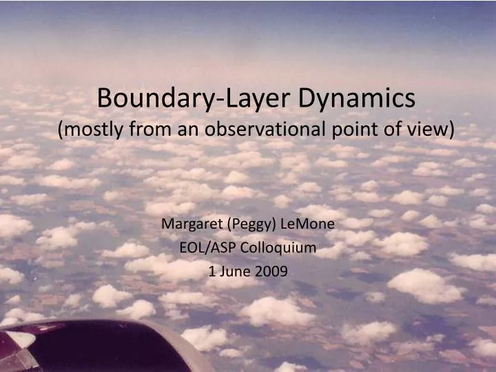
Boundary-Layer Dynamics (mostly from an observational point of view). Margaret (Peggy) LeMone EOL/ASP Colloquium 1 June 2009. REFERENCES: Numerous field programs 2 types: Focus on PBL structure/dynamics/turbulence (AHATS)

E N D
Boundary-Layer Dynamics(mostly from an observational point of view) Margaret (Peggy) LeMone EOL/ASP Colloquium 1 June 2009
REFERENCES: Numerous field programs 2 types: Focus on PBL structure/dynamics/turbulence (AHATS) PBL component of more comprehensive experiment (GATE, hurricanes) EARLY: O’Neill, Nebraska (“Exploring the Atmosphere’s First Mile”, Lettau and Davidson (1957) The “Kansas Experiment” (1968, SW Kansas) MORE RECENT Puerto Rico (1972) AMTEX (1975) GARP Atlantic Tropical Experiment (GATE, E Tropical Atlantic Ocean, Summer 1974) STORM Fronts Experiment Systems Test (NE Kansas, Spring1992) CASES-97 (SE Kansas, Spring 1997) CASES-99 (SE Kansas, Fall 1999) ACE (Atmospheric Chemistry Experiment (West of Tasmania, Dec. 1995) IHOP_2002 (Southern Great Plains, late Spring 2002) WKY-TV Tower (Oklahoma, year round, until 1980s) CCOPE (Cooperative Convective Precipitation Experiment, Montana, 1981) T-REX (Terrain-Induced Rotor Experiment, Owens Valley, California, 2006) STAAARTE (Switzerland, 1999) AND – modeling studies as well.
Definition of “Boundary Layer” When you take off or land in an airplane, the air is “bumpy” near the ground but gets smooth higher up. The “bumpy” layer near the ground is the daytime planetary boundary layer (convective boundary layer) Which leads to the AMS Glossary of Meteorology Definition (paraphrased), the layer of air near the ground that is directly affected by friction from the ground and possibly by transport of heat from the surface.
Different “Views” of the Convective Boundary Layer = 10 km horizontally 64 km along perimeter of 60-km circle Lidar aerosol backscatter over the Pacific, west of Tasmania (Donald Lenschow) 23 km N-S WCR radar reflectivity (insects) in dry CBL 29 May 2002, OK, (Bart Geerts). 49 km E-W DIAL Lidar water vapor and vertical velocity in dry CBL IHOP_2002, 7 June 2002, OK (Chris Kiemle et al., 2007, JTech)
Vertical Distribution of Turbulence in CBL Turbulence kinetic energy = u2+ v2+ w2, where the lower-case letters indicate a departure from the mean, is elevated through the CBL.. u2 and v2 maximum near the surface; w2 maximum within PBL. U, V = horizontal wind; W = vertical wind, w* is a scaling velocity: zi = PBL depth. Lenschow et al. (1980, AMTEX, JAS
Idealized PBL (1960s, pre-LES) Force balance above CBL (Northern Hemisphere) PGF wind vector H Coriolis + centrifugal L Force balance in CBL (Northern Hemisphere) Friction Coriolis + centrifugal • Wind at top of PBL along • isobars (normal to pressure • gradient). • Wind at surface is • slower, • toward low pressure • Slowdown by friction reduces Coriolis • and centrifugal effects. Wind hodograph in neutral PBL (Moeng and Sullivan, JAS, 1994) Potential temperature and mixing ratio well-mixed
Vertical Structure – Idealized CBL(strong convective heating from the bottom, supported by LES) Force balance above CBL (Northern Hemisphere) PGF Coriolis + centrifugal PGF Force balance in CBL (Northern Hemisphere) Friction Coriolis + centrifugal Change in force balance with height, leads to wind turning takes place in the entrainment layer
Surface Layer (M-O theory, Paulson 1970, updated) (blue=log profile) (red=stability correction) Stable Neutral Unstable Figure from Fleagle and Businger, 1963, Adapted from Lettau and Davidson, 1957, Exploring the Atmosphere’s Lowest Mile)
Semi-Idealized Equations for Wind and Virtual Potential Temperature Virtual potential temperature Qv Horizontal wind components U and V aligned such that Overbars and capital letters indicate averages Assuming horizontal heterogeneity and no change in wind…
CONVECTIVE BOUNDARY LAYER Assume horizontal heterogeneity wind steady state U, V and Qv well-mixed vertically no sources/sinks for Qv
Convective Boundary Layer Similarly and ≈ 0 = 0 or Fluxes vary linearly with height. C1, C2, and C3are constants
TOP: Idealized LEFT: LES (shading) with observations 10 Sept 1974 (GATE)1 RIGHT: Observed vertical flux of along- wind component of momentum2 -0.04 0.0 0.08 0.16 0.24 1Nicholls et al. (GATE, 1982, QJRMS); 2Pennell and LeMone (Puerto Rico,1974, JAS)
For fair weather, light winds, w’qv‘ at h ≈-0.2 w’qv‘ at surface CAUTION: The “-0.2” rule applies to w’qv’ not w’qv’ h Normalized virtual temperature flux for four fair-weather days in GATE.2 Note that mixing-ratio and humidity-flux profiles remain linear, but with varying slopes. 10 Sept 1974 (Day 253, GATE) temperature-flux profile, tropical East Atlantic1 1Nicholls et al. (1982, QJRMS) 2Nicholls and LeMone (1980, JAS)
Exception: growing PBL with strong shear at PBL top (Conzemius and Fedorovich, 2006)
How well does wind fit mixed-layer model? OVER LAND (Oklahoma example) Less shear daytime Low-shear occur local noon to early afternoon OVER OCEAN (Tropical BL) Six-month average: 2 m/s increase with height 6° veering with height (Gray 1972)
An exception: rapidly-growing PBL Nice mixed layer for 10 March, but not for 27 February. Horizontal advection and wind above PBL similar. Shear on 27 Feb from rapid engulfment of strong northerly momentum as PBL grew in bottom example. LeMone et al. (1998, BLM, STORM-FEST)
IMPACT OF SURFACE HETEROGENEITY:DATA SOURCE: 50-km flight track + surface array SE of Wichita, Kansas 8 8 9 9 Winter Wheat (brown) + + + + Grassland (tan, light green) G 7 7 + + 1 May 97 (CASES) 1 May 97 (CASES) WW 7-9 on grassland A 28 May 02 (IHOP) 16 May 02 (IHOP) A’ 12 June 02 (IHOP) 14 June 02 (IHOP) Winter Wheat Harvested ~ 15 June
Impact of Surface Heterogeneity IHOP_2002 (Summer) A’ Land-use map Red line = flight track Oranges, pinks: crops Light green: grassland Summer (IHOP) Wheat dormant (warm) Grass green (cool) H larger over/downstream of winter wheat Fluxes are 4-km running averages plotted every kilometer. A Longitude
Impact of Surface Heterogeneity for CASES-97 (spring) 37.5 37.4 A’ 37.3 A A and A’ – green winter wheat (brown in map) Green and Tan – Grass (mixed dormant and green) H larger over/downstream of winter wheat Also – with super-adiabatic lapse rate, higher elevations have higher temperatures than surrounding air at same height.
Heterogeneous surface effect on horizontal winds RWP 1-hour “Consensus” winds Whitewater Beaumont COOL WARM Oxford Wind (SSW 5-6 m s-1) LeMone et al. BLM 2002
IMPACT on BL STRUCTURE:Mesoscale Circulations in CASES-97 Large-scale subsidence Q for Eastern Track and “Triangle Legs” Aircraft conv/div patterns ABLE Radar wind profiles Green fetch cool air Dormant fetch + elevated heat source (fetch along ridge) Warm air
Heterogeneity at the top of the PBL – Cloudsheterogeneous cloud distribution • Wind + stability conditions imply • horizontal roll vortices over region to • right • Clouds streets visible only over land • (LCL high enough for clouds to form). • Similarly • Over Ocean, clouds reveal islands • Over land • Differences in land cover affect cloud • distribution1 • First clouds over harvested winter • wheat field in Oklahoma • Suppressed clouds over and around • lakes • Clouds/storms form preferentially over • elevated terrain • 1Rabin et al (BAMS, 1990) 1 Gemini image of cloud streets over Georgia coast.
Heterogeneity at the top of the PBL – Cloudsheterogeneous cloud distribution 1 • Over land • Differences in land cover affect cloud • distribution1 • First clouds over harvested winter • wheat field in Oklahoma • Suppressed clouds over and around • lakes • Clouds/storms form preferentially over • elevated terrain Cumulus clouds forming over foothills west of Boulder – there were no clouds anywhere else. 1Rabin et al (BAMS, 1990)
Low shear Cumulus draw air from beneath via buoyancy-generated pressure forces (solenoidal circulation) Large vertical shear at cloud base Pressure forces generated by interaction of updraft with shear (as well as buoyancy). Buoyant Where p’ = p0sin(2p/L) w’ = -w0cos(2p/L) p’ and w’ are departures from layer means. Complete Equation: (Rotunno and Klemp, MWR, 1982)
Cumulus increase subcloud vertical-velocity variance • (relative to clear-sky values) AMTEX data and formula from Lenschow et al. (JAS)
Modulation of PBL by waves (local origin) • Cu generate waves • Waves assume characteristics determined by lower-tropospheric environment • Waves modulate PBL behavior Latitude (Degrees North) 9.4 Waves generated from other sources can also modulate PBL motions. 8.4 23.4 23.0 22.6 Schematic: Based on Clark et al. (1986) Data: LeMone and Meitin (1984) Longitude (Degrees West)
The Growing PBL (14 June 2002, Oklahoma Panhandle) Figure 8, Bennett et al., to be submitted to MWR.
The Growing PBL PBL top growth change: results from heating from below, entrainment of air from above the boundary layer, represented by entrainment velocity we in response to buoyancy flux and mechanical mixing BL grows against subsiding air, represented by mean vertical velocity W Surface virtual temperature flux Bennett et al. (MWR, submitted, IHOP_2002)
VERY idealized growth rate, for little shear at PBL top, no advection DQ Where h is PBL depth Dz=Dh ≡ g is the gradient above h (no heat mixed in from above PBL, i.e., no entrainment) Thus, for constant flux, h ~ t1/2. Note that here there is no entrainment Growth by “encroachment”
Entraining PBLs (still no shear) from Garratt (1992) Start with two relationships: No entrainment (b=DQv=0) Obtain: Qvm Qv With entrainment: (same as previous slide) Conzemius and Fedorovich (2006, JAS) discuss importance of shear; and note that a value less than -0.2 for the ratio of buoyancy flux at h to that at the surface is an indication of the importance of shear.
4:00 8:00 12:00 16:00 20:00 18 0 6 12 18 Signal-to-Noise Ratio T.L. h stable layer top super-adiabatic layer top 6:30 7:59 9:29 12:29 14:00 15:30 17:00 18:33 20:22 21:30 10:59 CASES-97
Data: CASES-99, from S. Burns Nocturnal PBL 1200 LST 2000 LST (Schematic from Garratt (1992) At night, cooling due to IR radiation. Surface cools most rapidly.
Nocturnal PBL: Turbulence not necessarily decrease with height “upside-down” BL “z-less” BL Poulos et al. (BAMS, 2003, CASES-99)
Airflow at night can decouple from mean flow if sufficiently stable, or sufficiently large. Clear nights with light wind: Air at low levels decoupled from synoptic flow. Cooling negative buoyancy and downhill flow. Air current flowing downhill continues to cool, creating a linear dependence of temperature with elevation in the descending current. Windy Nights Near-surface air coupled to synoptic flow (constant potential temperature) Intermediate: Near-surface air intermittently decoupled from synoptic flow. Top (Mahrt et al. BLM, 2001, CASES-99), Bottom (LeMone et al. JAS, 2002, CASES-97). Also see Acevedo and Fitzjarrald, JAS, 2001)
Complex Terrain: ABL affected by the presence of terrain-forced and diurnal flows at many spatial and temporal scales Example of conceptual model of fair weather evolution of ABL in mountains: NIGHT DAY Whiteman, 2000, after Fiedler, from de Wekker
Daytime PBL – Complex Terrain (aerosols as tracers) AL height 1: mountain venting (elevated heat source) 2: cloud venting (clouds draw in air from below) 3: advection (local and from elsewhere) CBL height (De Wekker) De Wekker et al, 2004
Outstanding Research Problems for PBL (only a subset) • How to measure (at the surface): Surface energy budget, transfer of trace gases • How to measure (at the PBL top): PBL top, entrainment rate, vertical velocity • Interaction of PBL with cumulus and stratiform clouds • Anything to do with nocturnal/stable PBLs • Behavior of turbulence at small scales • Surface energy budget in complex terrain (on a slope) • Effects of surface heterogeneity • (surface properties, terrain, ocean waves, cities, wind farms, solar farms) • Dispersion of aerosols, trace gases (especially for complex terrain, stable conditions) • Interaction of mesoscale phenomena (waves, PBL mesoscale circulations) • with PBL turbulence and fluxes • Effects of chemical reactions on PBL flux and concentration profiles • Representation in models of • surface layer (over land and ocean, especially in strong winds • PBL • Sub-grid turbulence • The role of PBL in the evolution of precipitation convection • (onset of convection through “recovery” of boundary layer) • Behavior of the PBL during the “evening transition”
References Carson, D.J., 1973: The development of a dry inversion-capped convectively unstable boundary layer. Q. J. Roy. Meteor. Soc., 99, 450-467. Conzemius, R.G., and E. Fedorovich, 2006: Dynamics of sheared convective boundary layer entrainment, Part I: Methodological background and large-eddy simulation. J. Atmos. Sci., 63, 1151-1178. Garratt, J. The Atmospheric Boundary Layer, Cambridge University Press, 1992. And articles referred to on the individual pages.