Download
1 / 17
170 likes | 461 Views
Observational study of the transition from unbroken marine boundary layer stratocumulus to the shallow cumulus regime. Irina Sandu and Bjorn Stevens Max-Planck-Institut für Meteorologie KlimaCampus, Hamburg . Motivation.

E N D
Observational study of the transition from unbroken marine boundary layer stratocumulus to the shallow cumulus regime Irina Sandu and Bjorn Stevens Max-Planck-Institut für Meteorologie KlimaCampus, Hamburg
Motivation Cloud regimes ranging from stratocumulus in the subtropics, to shallow cumuli and deep convective clouds toward the Equator (Fig. 1 Stevens, 2005b, following Arakawa (1975)). Aqua Images NE Pacific SE Pacific
So far ? Observations: Albrecht, 1995, subsequent studies based on ASTEX (1992) , Pincus et al. 1997 Theory and modeling: Bretherton et al., 1992, 1997,1999, Krueger et al. 1995, Wyant et al. 1997 (Bretherton et al., 1992)
So far ? Observations: Albrecht, 1995, subsequent studies based on ASTEX (1992) , Pincus et al. 1997 Theory and modeling: Bretherton et al., 1992, 1997,1999, Krueger et al. 1995, Wyant et al. 1997 Now ?Last generation satellites (MODIS, MSG, etc.)ECMWF ERA-INTERIM re-analysisImproved LES models (or at least more powerful computers) Aim Use satellite data and NWP reanalysis to develop a statistical view of the transition between stratocumulus and shallow cumuli
Our questions Do the data show a transition from Sc. to Cu.? How frequently does it occur? Is it different from one region to another? How is it related to the large scale factors?
Methodology Trajectories + Re-analysis + Satellite data How ? MODIS (Terra, Aqua) AMSR-E HYSPLIT (ERA-INTERIM) ERA-INTERIM 2002-2007 (May to October in NE, July to December SE) Starting time: 11 LT, Duration: 6 days, Height: 200m When ? Where ? Klein&Hartmann (1993) zones : NE/SE Atlantic, NE/SE Pacific NEP NEA SEA SEP
Data sets • ERA-INTERIM: • latest ECMWF reanalysis (from 2002) • 1.5 X 1.5 degrees, every 6 hours • SST, , qt, LTS, D , LE, H, CF, AOD • MODIS: • Terra (10.30 LT) and Aqua (13.30 LT) (from 2002/2003) • L3 products:1 X 1 degrees • Liquid Water cloud fraction, LWP, optical thickness, effective radius • AMSR-E: • Aqua (1.30 and 13.30 LT) (from 2003) • 0.25 X 0.25 degrees • LWP, TWP, SST, precipitation • GPCP: • daily means of precipitation rate • 1 X 1 degrees
Some statistics Total number of trajectories Trajectories going over warmer waters (SW in NE NW in SE) 30% of the total number of trajectories, having the biggest initial CF, i.e a CF superior to For the subsequent analysis we consider the 30% of the total number of trajectories having the biggest CF (initially) and going over warmer waters
Probability distribution of the selected trajectories ending point (%) NEA NEP * * * * * * * * * * * * * * * * * * + 6 days + 6 days SEA SEP + 6 days + 6 days * * * * * * * * * * * * * * *
The average trajectory + CF MODIS Terra (10.30 am) NEA NEP < < < < < < SEA SEP < < < < <
Cloud fraction along the trajectories in the 4 zones CF MODIS
Variables along the trajectories in the 4 zones (I) LWP AMSR-E PP GPCP CF MODIS SST LTS D
Variables along the trajectories in the 4 zones (II) 700 WATER VAPOR qt700
Mean July trajectory (NEA)(from mean July day, mean July fields) Which is the difference between the transition along streamlines versus the transition composited over trajectories?
Mean July trajectory (NEA)(from mean July day, mean July fields) composite - - - - streamline LTS D SST
In summary There is a transition, between 1 and 3 days downstream of the maximum cloudiness The transitions are characterized by a sharp reduction in cloudiness, increased variability in cloud fraction among trajectories The transition is similar in the 4 basins, hence it makes sense to think of a generic transition Properties of the generic transition: increasing SST, constant divergence ?, constant 700, increasing qt 700 increased surface fluxes + decreased radiative cooling at cloud top, which supports Bretherton’s theory, the flow gradually becomes more surface driven Next: modeling study to explore these ideas, a possible intercomparison case