Download
1 / 41
410 likes | 543 Views
ECE 3317. Prof. Ji Chen. Spring 2014. Notes 6 Transmission Lines ( Time Domain). Note about Notes 6. Note:

E N D
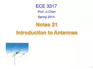
ECE 3317 Prof. Ji Chen Spring 2014 Notes 6 Transmission Lines(Time Domain)
Note about Notes 6 Note: Transmission lines is the subject of Chapter 6 in the Shen & Kong book. However, the subject of wave propagation in the time domain is not treated very thoroughly there. Chapter 10 of the Hayt book has a more thorough discussion.
Transmission Lines a b z A transmission line is a two-conductor system that is used to transmit a signal from one point to another point. Two common examples: Twin lead Coaxial cable A transmission line is normally used in the balanced mode, meaning equal and opposite currents (and charges) on the two conductors.
Transmission Lines (cont.) Here’s what they look like in real-life. Coaxial cable Twin lead
Transmission Lines (cont.) CAT 5 cable (twisted pair)
Transmission Lines (cont.) E - l - - + + + + + - + - - -l Some practical notes: • Coaxial cable is a perfectly shielded system (no interference). • Twin line is not a shielded system – more susceptible to noise and interference. • Twin line may be improved by using a form known as “twisted pair” (e.g., CAT 5 cable). This results in less interference. E Twin lead Coax
Transmission Lines (cont.) Another common example (for printed circuit boards): w r h Microstrip line
Transmission Lines (cont.) Transmission lines are commonly met on printed-circuit boards. Microstrip line A microwave integrated circuit (MIC)
Transmission Lines (cont.) Microstrip line
Transmission Lines (cont.) Transmission lines commonly met on printed-circuit boards w er h er h w Microstrip Stripline w w w er h er h Coplanar waveguide (CPW) Coplanar strips
Transmission Lines (cont.) Symbol for transmission line: + - z 4 parameters Note: We use this schematic to represent a general transmission line, no matter what the actual shape of the conductors.
Transmission Lines (cont.) z Four fundamental parameters that characterize any transmission line: These are “per unit length” parameters. 4 parameters Capacitance between the two wires C= capacitance/length [F/m] L= inductance/length [H/m] R= resistance/length [/m] G= conductance/length [S/m] Inductance due to stored magnetic energy Resistance due to the conductors Conductance due to the filling material between the wires
Circuit Model Dz z RDz LDz CDz GDz + - Circuit Model: z Dz
Coaxial Cable a b z Example (coaxial cable) d= conductivity of dielectric [S/m] m= conductivity of metal [S/m] (skin depth of metal)
Coaxial Cable (cont.) E - l - - + + + + + - + - - -l Overview of derivation: capacitance per unit length a b
Coaxial Cable (cont.) y x E Js Overview of derivation: inductance per unit length a b
Coaxial Cable (cont.) Overview of derivation: conductance per unit length RC Analogy: a b
Coaxial Cable (cont.) Relation Between L and C: Speed of light in dielectric medium: This is true for ALL transmission lines. Hence: ( A proof will be seen later.)
Telegrapher’s Equations RDz LDz I(z+Dz,t) I(z,t) + V(z+Dz,t) - + V(z,t) - CDz GDz z z+Dz z Apply KVL and KCL laws to a small slice of line:
Telegrapher’s Equations (cont.) Hence Now let Dz 0: “Telegrapher’s Equations (TEs)”
Telegrapher’s Equations (cont.) • Take the derivative of the first TE with respect to z. • Substitute in from the second TE. To combine these, take the derivative of the first one with respect to z:
Telegrapher’s Equations (cont.) Hence, we have: There is no exact solution to this differential equation, except for the lossless case. The same equation also holds for i.
Telegrapher’s Equations (cont.) Lossless case: “wave equation” Note: The current satisfies the same differential equation. The same equation also holds for i.
Solution to Telegrapher's Equations Hence we have Solution: where f andg arearbitrary functions. This is called the D’Alembert solution to the wave equation (the solution is in the form of traveling waves). The same equation also holds for i.
Traveling Waves Proof of solution General solution: It is seen that the differential equation is satisfied by the general solution.
Traveling Waves (cont.) f (z) z t = 0 t = t2 > t1 t = t1 > 0 V(z,t) z z0 z0 + cdt1 z0 + cdt2 Example (square pulse): t = 0 z0 “snapshots of the wave”
Traveling Waves (cont.) g (z) z Example (square pulse): t = 0 z0 “snapshots of the wave” t = t1 > 0 t = t2 > t1 t = 0 V(z,t) z z0 - cdt1 z0 - cdt2 z0
Traveling Waves (cont.) Loss causes an attenuation in the signal level, and it also causes distortion (the pulse changes shape and usually gets broader). V(z,t) t = 0 t = t1 > 0 t = t2 > t1 z z0 z0 + cdt1 z0 + cdt2 (These effects can be studied numerically.)
Current Our goal is to now solve for the current on the line. (first Telegrapher’s equation) Lossless Assume the following forms: The derivatives are:
Current (cont.) This becomes Equating like terms, we have Hence we have Note: There may be a constant of integration, but this would correspond to a DC current, which is ignored here.
Current (cont.) Observation about term: Define the characteristic impedance Z0 of the line: The units of Z0 are Ohms. Then
Current (cont.) General solution: For a forward wave, the current waveform is the same as the voltage, but reduced in amplitude by a factor of Z0. For a backward traveling wave, there is a minus sign as well.
Current (cont.) Picture for a forward-traveling wave: forward-traveling wave z + -
Current (cont.) Physical interpretation of minus sign for the backward-traveling wave: backward-traveling wave z + - The minus sign arises from the reference direction for the current.
Coaxial Cable Example: Find the characteristic impedance of a coax. a z b
Coaxial Cable (cont.) a z b (intrinsic impedance of free space)
Twin Lead d a = radius of wires
Twin Line (cont.) These are the common values used for TV. 75-300 [] transformer 75 [] coax 300 [] twin line Twin line Coaxial cable
Microstrip Line w r h Parallel-plate formulas:
Microstrip Line (cont.) t = strip thickness More accurate CAD formulas: Note: The effective relative permittivity accounts for the fact that some of the fields are outside of the substrate, in the air region. The effective width w' accounts for the strip thickness.
Some Comments • Transmission-line theory is valid at any frequency, and for any type of waveform (assuming an ideal straight length of transmission line). • Transmission-line theory is perfectly consistent with Maxwell's equations (although we work with voltage and current, rather than electric and magnetic fields). • Circuit theory does not view two wires as a "transmission line": it cannot predict effects such as single propagation, reflection, distortion, etc. One thing that transmission-line theory ignores is the effects of discontinuities (e.g. bends). These may cause reflections and possibly also radiation at high frequencies, depending on the type of line.