Download
1 / 38
410 likes | 632 Views
ECE 3317. Prof. Ji Chen. E. x. Spring 2014. ocean. Notes 15 Plane Waves. z. Introduction to Plane Waves. A plane wave is the simplest solution to Maxwell’s equations for a wave that travels through free space.

E N D
ECE 3317 Prof. Ji Chen E x Spring 2014 ocean Notes 15 Plane Waves z
Introduction to Plane Waves • A plane wave is the simplest solution to Maxwell’s equations for a wave that travels through free space. • The wave does not requires any conductors – it exists in free space. • A plane wave is a good model for radiation from an antenna, if we are far enough away from the antenna. x E S z H
The Electromagnetic Spectrum http://en.wikipedia.org/wiki/Electromagnetic_spectrum
TV and Radio Spectrum AM Radio: 520-1610 kHz VHF TV: 55-216 MHz (channels 2-13) Band I : 55-88 MHz (channels 2-6) Band III: 175-216 MHz (channels 7-13) FM Radio: (Band II) 88-108 MHz UHF TV: 470-806 MHz (channels 14-69) Note: Digital TV broadcast takes place primarily in UHF and VHF Band III.
Vector Wave Equation Start with Maxwell’s equations in the phasor domain: Faraday’s law Ampere’s law Assume free space: Ohm’s law: We then have
Vector Wave Equation (cont.) Take the curl of the first equation and then substitute the second equation into the first one: Define: Wavenumber of free space [rad/m] Then Vector wave equation
Vector Helmholtz Equation Recall the vector Laplacian identity: Hence we have Also, from the divergence of the vector wave equation, we have: Note: There can be no charge density in the sinusoidal steady state, in free space (or actually in any homogenous region of space).
Vector Helmholtz Equation (cont.) Hence we have: Vector Helmholtz equation Recall the property of the vector Laplacian in rectangular coordinates: Reminder: This only works in rectangular coordinates. Taking the x component of the vector Helmholtz equation, we have Scalar Helmholtz equation
Plane Wave Field z Assume The electric field is polarized in the x direction, and the wave is propagating (traveling) in the z direction. y E x Then or For wave traveling in the negative z direction: Solution:
Plane Wave Field (cont.) For a plane wave traveling in a lossless dielectric medium (does not have to be free space): where (wavenumber of dielectric medium)
Plane Wave Field (cont.) The electric field behaves exactly as does the voltage on a transmission line. Notational change: All of the formulas that we had for a transmission line now hold for a transmission line, using this notation change. Example:
Plane Wave Field (cont.) For a lossless transmission line, we have: For a plane wave, we have: A transmission line filled with a dielectric material has the same wavenumber as does a plane wave traveling through the same material. A wave travels with the same velocity on a transmission line as it does in space, provided the material is the same. same
Plane Wave Field (cont.) The H field is found from: so
Intrinsic Impedance or so Hence where Intrinsic impedance of the medium Free-space:
Poynting Vector For a wave traveling in a lossless dielectric medium: The complex Poynting vector is given by: Hence we have (no VARS)
Phase Velocity Phasor domain: Time domain: From our previous discussion on phase velocity for transmission lines, we know that Hence we have so (speed of light in the dielectric material) • Notes: • All plane wave travel at the same speed in a lossless medium, regardless of the frequency. • This implies that there is no dispersion, which in turn implies that there is no distortion of the signal.
Wavelength From our previous discussion on wavelength for transmission lines, we know that Hence For free space: Also, we can write Hence Free space:
Summary (Lossless Case) z S y H E x Time domain:
Lossy Medium Return to Maxwell’s equations: E x ocean Assume Ohm’s law: Ampere’s law z We define an effective (complex) permittivity c that accounts for conductivity:
Lossy Medium (cont.) Maxwell’s equations: then become: The form is exactly the same as we had for the lossless case, with Hence we have (complex) (complex)
Lossy Medium (cont.) Examine the wavenumber: Note: The complex effective permittivity lies in the fourth quadrant. Principal branch: Denote: Using the principal branch of the square root, the wavenumber klies in the fourth quadrant. Hence: Compare with lossy TL:
Lossy Medium (cont.) (choose E0 = 1) The “depth of penetration” dpis defined.
Lossy Medium (cont.) The complex Poynting vector is:
Example Ocean water: (These values are fairly constant up through microwave frequencies.) Assume f= 2.0 GHz
Example (cont.) fdp [m] 1 [Hz] 251.6 10 [Hz] 79.6 100 [Hz] 25.2 1 [kHz] 7.96 10 [kHz] 2.52 100 [kHz] 0.796 1 [MHz] 0.262 10 [MHz] 0.080 100 [MHz] 0.0262 1.0 [GHz] 0.013 10.0 [GHz] 0.012 100 [GHz] 0.012 The depth of penetration into ocean water is shown for various frequencies. Note: The relative permittivity of water starts changing at very high frequencies (above about 2 GHz), but this is ignored here.
Loss Tangent Denote: The loss tangent is defined as: The loss tangent characterizes how lossy the material is. We then have:
Loss Tangent The loss tangent characterizes how fast the plane wave decays relative to a wavelength. tan << 1: low-loss medium (attenuation is small over a wavelength) tan >> 1: high-loss medium (attenuation is large over a wavelength)
Low-Loss Limit: tan << 1 The wavenumber may be written in terms of the loss tangent as Low-loss limit: (independent of frequency) or
Low-Loss Limit: tan << 1 fdp [m] tan Ocean water 1 [Hz] 251.6 8.88108 10 [Hz] 79.6 8.88107 100 [Hz] 25.2 8.88106 1 [kHz] 7.96 8.88105 10 [kHz] 2.52 8.88104 100 [kHz] 0.796 8.88103 1 [MHz] 0.262 888 10 [MHz] 0.080 88.8 100 [MHz] 0.0262 8.88 1.0 [GHz] 0.013 0.888 10.0 [GHz] 0.012 0.0888 100 [GHz] 0.012 0.00888 Low-loss region
Polarization Loss The permittivity can also be complex, due to molecular and atomic polarization loss (friction at the molecular and atomic levels) . Example: distilled water: 0 (but it heats up well in a microwave oven!). Notation: (complex permittivity)
Polarization Loss (cont.) Note: In practice, it is usually difficult to determine how much of the loss tangent comes from conductivity and how much comes from polarization loss.
Summary of Permittivity Formulas Note: If there is no polarization loss, then
Polarization Loss (cont.) Complex relative permittivity for pure (distilled) water
Polarization Loss (cont.) For modeling purposes, we can lump the polarization losses into an effective conductivityterm and pretend that the permittivity is real: Note: In most measurements involving heating, we cannot tell if loss is really due to conductivity or polarization loss. where
Polarization Loss (cont.) Practical note: • For some materials, it is the conductivity that is approximately constant with frequency. Ocean water: 4 [S/m] • For other materials, it is the loss tangent that is approximately constant with frequency. Teflon: tan 0.001
Note on Notation Be careful: Most books do not use the notation c. They often use only the notation . • Sometimes it means • Sometimes it means c. Our notation: Usual notation: