Download
1 / 45
450 likes | 568 Views
The Designs and Analysis of a Scalable Optical Packet Switching Architecture. Speaker: Chia-Wei Tuan Adviser: Prof. Ho-Ting Wu 3/4/2009. Outline. Introduction Switching Architecture and Control Strategies Performance Results Input Traffic Model Queueing Analysis

E N D
The Designs and Analysis of a Scalable Optical Packet Switching Architecture Speaker: Chia-Wei Tuan Adviser: Prof. Ho-Ting Wu 3/4/2009
Outline • Introduction • Switching Architecture and Control Strategies • Performance Results • Input Traffic Model • Queueing Analysis • Numerical Results for Queueing Analysis Model
Outline • Introduction • Switching Architecture and Control Strategies • Performance Results • Input Traffic Model • Queueing Analysis • Numerical Results for Queueing Analysis Model
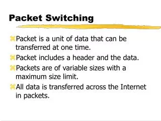
Contention resolution in switches • Contention resolution is an important issue when several packets contend for a common network resource. • When two input packets are destined for the same output port simultaneously, packet contention occurs. • When contention occurs, storing packets into the switch buffers becomes the most general technique.
Contention resolution in switches • At present, optical storage technology is not available. • Thus, switching operations are done electronically, forcing the optical signal to be converted to an electronic format. • But, in all-optical networks, packets are switched optically until they reach their destination. • That is, switching must also be optical in all-optical networks.
How to store packetsin all-optical networks? • Switched delay lines (SDL). • Storing of packets in fiber DLs act as transient optical buffers. • Quadro is a single-buffer DL switching architecture. • M-Quadro is a multi-buffer Quadro architecture that uses a longer DL to increase the buffering capacity.
Outline • Introduction • Switching Architecture and Control Strategies • Performance Results • Input Traffic Model • Queueing Analysis • Numerical Results for Queueing Analysis Model
B-Quadro Switching Architecture • The length of DLi is mi. • The (m2-m1)th slot in DL2 counting from left to right is termed “virtualslot” , if m2 > m1.
Left control strategy (LCS) • Ex1: • LCS applied:
Right control strategy (RCS) • Ex2: • RCS applied:
Virtual-slot control strategy (VCS) • VCS is to ensure, whenever possible, that outgoing state 1 be different from outgoing state 2. • Deflection: • Internal blocking:
Virtual-slot control strategy (VCS) • Ex1: • VCS applied:
Virtual-slot control strategy (VCS) • Ex2: • VCS applied:
The limitations of M-Quadro • Ex3: • VCS applied:
The M-B-Quadro Architecture • The packets through the bypass line (BL) are carried without delay. (No buffering capability)
Example of M-B-Quadro • Ex3: • LAVS applied:
Multi-stage Multi-buffer Bypass Quadro (M2-B-Quadro) Switch Architecture • 3 x 3 switch: • n x n switch:
Outline • Introduction • Switching Architecture and Control Strategies • Performance Results • Input Traffic Model • Queueing Analysis • Numerical Results for Queueing Analysis Model
The Comparsion between M-Qdadro and M-B-Qdadro with Symmetrical Traffic
The Parameter of Asymmetrical Traffic • The load of each input is ρ. • Let X be a random variable that indicates the state of a input port. • P(X=i) represents the probability of the packet destined for output port i at specific time slot. • P(X=0) = 1- ρ. • P(X=1) = R1* ρ. • P(X=2) = R2* ρ. • where Ri is the ratio of total packets to the packets destined for output port i.
The Comparsion between M-Qdadro and M-B-Qdadro with Nonbursty and Asymmetrical Traffic
The Comparsion between M-Qdadro and M-B-Qdadro with Bursty and Asymmetrical Traffic
Outline • Introduction • Switching Architecture and Control Strategies • Performance Results • Input Traffic Model • Queueing Analysis • Numerical Results for Queueing Analysis Model
Bursty Traffic Model • Pa: The probability of no packet arriving in the next slot, given the current slot is idle. • Pb: The probability of the next arrival will be part of the burst. (i.e., destined to the same destination).
The properties of Bursty Traffic Model • Expected bursty length = • Offered load at each input port =
Asymmetric Traffic Model • In realistic networks, the traffic is not only bursty but also asymmetric. Back to P32
How to determine the value of P01 and P02? • Calculus the steady state distribution: • P(X=i) can be derived by summing the steady-state probability in {bursty1, destination i} and {bursty2, destination i} states. • After rearranging, we obtain: Back to P32
Outline • Introduction • Switching Architecture and Control Strategies • Performance Results • Input Traffic Model • Queueing Analysis • Numerical Results for Queueing Analysis Model
Exact Analytical Model • is the state (i.e., destination) of slot j at DL i. • The state of input port i is represented as xi. • The state definition of exact DTMC.
Control Strategies • Let and are two instances of . • Define control strategy as , where is part of control strategy which determine the next incoming slot i. • Assuming is the next state of , the relation of them is:
State Transition Matrix In Non-bursty Traffic Case • In non-bursty traffic case, • Thus, state transition probability in can be reduced to • The non-bursty case can be further divided into • Symmetrical case: Set to 1/n for k=1,2,…, n. • Asymmetrical case: Set to some probability greater or smaller than 1/n for k=1,2,…, n
State Transition Matrix In Bursty Traffic Case • In bursty traffic case, it can also be further divided into • Symmetrical case: Set P(x=1) = P(x=2). • Asymmetrical case: Set P(x=1) ≠ P(x=2). • where is the transition probability in the traffic model diagram. in the equation
Calculus Steady State • Let be steady state distribution. where is the space size. • Compute iteratively until • Deflection probability:
Approximate Asymptotic Model • Goal: get the lowest bound of deflection probability. • Unlimited delay line size. • The approximate asymptotic model assume that m1 = m2 = … = mn-1 = 1 and mn = ∞.
Estimation • Redefine the state definition of DTMC as • Estimation: Back
An Iterative Method to calculus the steady state distribution • Initial: • Calculus state transition probability matrix:
An Iterative Method to calculus the steady state distribution • Calculus the next state distribution vectors. • Check the convergence condition. • If the condition holds, stop the program and compute deflection probability. • Otherwise, calculus the new estimate conditional probability and go to step 2)
Outline • Introduction • Switching Architecture and Control Strategies • Performance Results • Input Traffic Model • Queueing Analysis • Numerical Results for Queueing Analysis Model
Exact model and simulation for Symmetrical Traffic • M1=1, M2=4. • Using LAVS control strategy.
Exact model and simulation for Asymmetrical Traffic • M1=1, M2=4. • Using LAVS control strategy. • Expected bursty length = 20.
Lowest bound of deflection probability. • Under a specific traffic condition, we obtain the lowest bound of deflection prob. • bursty length = 5 and offered load = 0.6 :
Conclusions • M-B-Quadro can achieve lower packet deflection probability. • The analytical model can evaluate the system performances under non-bursty, bursty, symmetrical, and asymmetrical conditions. • The numerical results show the analytical model is successful to reveal the lowest bound of deflection probability in this switching architecture.
Reference • [1] Chlamtac, I. and Fumagalli, and Suh, C. J., 2000, “Multibuffer Delay Line Architecture for Efficient Contention Resolution in Optical Switching Nodes,” IEEE Transactions on Communications, Vol. 48, No. 12, pp. 2089- 2098. • [2] Haas, Z., 1993, “The Staggering Switch - An Electronically Controlled Optical Packet Switch,” IEEE/OSA Journal of Lightwave Technology, Vol. 11, No. 5/6, pp. 925-936. • [3] Wang-Rong Chang, Ho-Ting Wu, Kai-Wei Ke, and Hui-Tang Lin, “The Designs of a Scalable Optical Packet Switching Architecture”, Journal of the Chinese Institute of Engineers, vol. 31, no. 3, pp. 469-479, 2008.
Thank you! Q&A