Download
1 / 43
440 likes | 675 Views
Land-Surface Modeling. 19 November 2012. Thematic Outline of Basic Concepts. What are the physical processes that are relevant to land-surface modeling? How are these processes represented by a land-surface model?

E N D
Land-Surface Modeling 19 November 2012
Thematic Outline of Basic Concepts • What are the physical processes that are relevant to land-surface modeling? • How are these processes represented by a land-surface model? • How do land-surface models and data assimilation systems operate with atmospheric models?
Land-Surface Modeling • A land-surface model must be able to accurately depict the interactions of… • …the surface with the atmosphere • …the substrate with the surface • Here, we take the surface to refer to land and the substrate to refer to the sub-soil (sub-surface) layer. • Ocean modeling and air-sea interaction are important, but a separate, extensive set of lectures in their own right.
Land-Surface Modeling • Land-surface modeling requires the accurate representation of heat and moisture transfer within the surface and between it and the atmosphere. • Accurate atmospheric input to the surface is required for this to be achieved, however. • Land-surface modeling is thus best viewed as a coupled system between the atmosphere and surface.
Constructs for Land-Surface Modeling • Land-Surface Model (LSM) • Run simultaneously with an atmospheric model to predict primarily surface-atmosphere heat and moisture transfer. • Land Data Assimilation System (LDAS) • A standalone version of the LSM that synthesizes atmospheric inputs and surface information to predict the initial states of relevant land-surface fields. • Necessary for accurate atmospheric model initialization as such data are not routinely observed over wide areas.
Why Use an LDAS? • Necessary to spin-up realistic soil state fields. • True whether direct observations exist or not. • Akin to doing data assimilation for an atmospheric model. • Help to correct the initial estimates for soil state fields • Like atmospheric models, LSMs are imperfect! • Need to constrain soil state estimate to reality! • Note: when running a model, use the same LSM as was used to create the initial soil state fields! • Output from LSM may not work well with another LSM…
Land-Surface Modeling • LSM Input… • Land state variables (vegetation, soil moisture, soil temperature, topography, etc.) • Atmospheric information (winds, temperature, precipitation, radiative forcing) • LSM Output… • Surface latent and sensible heat fluxes • Reflected shortwave and emitted longwave radiation • Updated soil state (temperature and moisture) fields
Land-Surface Modeling surface substrate
Land-Surface Modeling • An LSM must be able to accurately simulate physical processes influencing heat and moisture transport… • …within the substrate • …along the surface-substrate interface • …along the atmosphere-surface interface • A full listing of relevant processes may be found on pgs. 172-174 of the text.
First Principles of LSMs Surface Energy Balance: R = LE + H + G R = net radiative forcing LE = latent heating H = sensible heating (surface<->atmosphere) G = sensible heating (substrate<->surface) Land-surface modeling deals with how to compute the land-surface terms of the surface energy budget.
First Principles of LSMs Radiative Forcing: Q = direct solar radiation incident at surface q = diffuse solar radiation incident at surface α = albedo (1-α = transmittance) I↑ = outgoing longwave radiation emitted by surface I↓ = absorbed longwave radiation emitted by atmosphere Note: typically computed by radiation parameterization
First Principles of LSMs Surface Water Budget: Θ = volumetric soil water content (dimensionless) P = precipitation, snowmelt, deposition, irrigation input ET = loss due to evapotranspiration RO = loss due to lateral runoff D = loss due to gravitational drainage to lower layers Land-surface modeling deals with how to compute the forcing terms of the surface water budget.
Second Principles of LSMs • Basic concepts: heat and moisture budget • Concepts influencing these budgets… • Vertical heat transport within the substrate • Vertical moisture transport within the substrate • Moisture transport within and by vegetation • We next describe the basic physics behind each of these concepts.
Vertical Heat Transport • Thermal Conductivity (ks): ability of the substance to transfer heat • Dependent upon soil composition (moisture content, density of soil vs. that of air, type of soil, etc.) • Heat Capacity (Cs): amount of heat required to raise the temperature of a unit volume by 1°C/1 K • Also dependent upon soil composition • Related: specific heat (cs), amount of heat required to raise the temperature of a unit mass by 1°C/1 K
Vertical Heat Transport • Thermal Diffusivity (Ks): ratio of thermal conductivity to the heat capacity (ks/Cs) • Controlling influence upon the rate of speed at which a temperature change propagates through a medium • Analogous to an exchange coefficient • Thermal Admittance (μs): the rate at which a surface can accept or release heat energy [μs = (ksCs)½] • Admittance of both the soil and atmosphere are important • Higher admittance = reduced temperature change because heat is transferred efficiently rather than stored locally
Vertical Heat Transport Moister soils require more thermal energy to warm by 1°C / 1 K than drier soils because of soil moisture dependence. thermal conductivity Moister soils have a greater ability to conduct heat because of soil moisture dependence. heat capacity thermal diffusivity thermal admittance Higher soil moisture content promotes a greater ability to transfer heat across a surface (rather than being trapped). Soil moisture dependence relies on ratio between increases in ks and Cs.
Vertical Heat Transport • Vertical heat transport in the substrate… • Primarily by conduction (molecular diffusion) • Down-gradient (from high to low) • Magnitude is proportional to that of the vertical temperature gradient and thermal conductivity, i.e., Hs = heat flux (positive upward) ks = soil thermal conductivity z = vertical coordinate (positive upward) Ts = substrate temperature
Vertical Heat Transport • Change of substrate temperature with time… • Change due to the vertical convergence of the heat flux: • If we make the approximation that thermal conductivity is constant with height within the substrate, we can write: Thus, Ts changes as a function of its second derivative with respect to depth and the thermal diffusivity (conductivity divided by capacity) of the soil.
Vertical Heat Transport • Daytime: warmer surface than substrate… • First derivative of Ts with height is positive. • Second derivative is also positive. • Because the first derivative is more positive at the top of the substrate than at the bottom. • With Ks positive-definite, Ts increases with time. • This results in a warming of the substrate with time.
Vertical Heat Transport • Nighttime: warmer substrate than surface… • First derivative of Ts with height is negative. • Second derivative is also negative. • Because the first derivative changes is more negative at the top of the substrate than at the bottom. • With Ks positive-definite, Ts decreases with time. • This results in a cooling of the substrate with time.
Application: Daily Temperature Oscillation • Manifestation of vertical extent of thermal transport: • The amplitude of the temperature oscillation decreases exponentially with increasing depth. amplitude at sfc. P = wave period (diurnal = 24 h, annual = 365 d) amplitude at z
Application: Temperature Oscillation daily annual Note deamplification of wave with increasing depth, increased depth over a longer duration, and time lag of maximum and minimum temperature with increasing depth.
Application: Temperature Oscillation • The amplitude of this oscillation is greater when… • Large conductivity (ks) • Small heat capacity (Cs) • If the exchange of heat from the atmosphere to the surface and substrate is large, the temperature oscillation is larger and penetrates deeper. • Further discussion: pg. 180 of the text. large thermal diffusivity
Vertical Water Transport • Five mechanisms, two applicable to water vapor and three to liquid water. • Those applicable to water vapor… • Convection: occurs if/when lapse rate of soil temperature exceeds the dry adiabatic lapse rate. Permits upward water vapor transport through dry soils via buoyant plumes. • Vapor Diffusion: down-gradient, molecular-level diffusion of water vapor. Proportional to soil water vapor content.
Vertical Water Transport • Changes in the height of the water table below the substrate • A water surface must be in dynamic equilibrium with its surrounding fluid. • Thus, local water excesses or deficits are reconciled by lateral water movement. • This can locally raise the water table where initially lower, or vice versa.
Vertical Water Transport height of water table
Vertical Water Transport • Surface-tension (molecular bonding/capillary) effects • Dependent upon soil moisture content and how well the soil can be permeated by water (porosity) • With stronger surface tension, water molecules are more strongly bound to soil particles. • Typically with wetter, less porous soils. • Permits water to gradually move upward via molecular attraction. • Generally manifest in the lower substrate, between the water table and the relatively dry layer above it. • Movement is typically from wetter to drier soils.
Vertical Water Transport • Downward infiltration from the surface • Driven by gravity, controlled by surface-tension, and influenced by the soils’ ability to retain water. • Water intake comes from rainfall, snowmelt, irrigation, etc. • Relevant definitions… • Hydraulic conductivity: ability of soil to transport water vertically; greatest when soil is wet and porous • Soil moisture potential: amount of energy needed to extract a given amount of water from a given type of soil (inverse of conductivity)
Water Transport by Vegetation • Influences the energy budget at the surface as well as the soil moisture content. • Relevant processes… • Extraction of substrate water by plants • Evaporation of surface water collected on the plant canopy • Transpiration of water vapor out of plant leaves’ pores • Largely dependent upon vegetation type and density, atmospheric moisture content, time of day/year, and heat and water stresses. • Physics behind transpiration are not well-understood, however.
Soil Moisture Budget • As we did for soil temperature, we now wish to express the soil moisture budget mathematically. • This expression will apply to subsurface layers and thus does not include direct effects of precipitation, evaporation, and runoff. • The surface soil moisture budget must include information about these import and export processes. • Mathematical manifestation: vertical moisture flux
Soil Moisture Budget Soil Moisture Budget: Θ = volumetric soil water content (dimensionless) Et = loss to plant canopy by evapotranspiration Liquid Water Mixing Ratio Tendency: KΘ = hydraulic conductivity (associated with infiltration) DΘ = soil water diffusivity (associated with surface-tension)
Soil Moisture Budget • Both KΘ and DΘ are highly non-linearly dependent upon soil moisture content and soil type. • Different models use different formulations; the example from the text is given by: Subscripts of s denote saturation values. b = empirically-derived coefficient Ψ = soil moisture potential Note dependence upon both soil moisture (via Θ) and soil type (parameters above).
Surface Energy Budget • General idea: transport from the surface to the atmosphere occurs via conduction (laminar sublayer). • Above the laminar sublayer, transport occurs via turbulent eddies. • We will effectively encapsulate both within our formulations for the surface heat and moisture fluxes. • Manifest via eddy (rather than molecular) diffusivities
Surface Energy Budget Surface sensible and latent heat fluxes: Ca = heat capacity of atmosphere cp = specific heat of atmosphere at constant pressure q = specific humidity KHa = diffusivity of heat in air KWa = diffusivity of moisture in air Subscripts of “ls” denote computation in laminar sublayer.
Surface Energy Budget Assumption: fluxes approximately constant with height DH = exchange coefficient for heat DW = exchange coefficient for moisture Both are integral functions of KH and KW with large dependence upon stability, wind speed, and surface roughness. Tg = ground temperatureTa = atmospheric temperature near the surface qs,sat = saturation specific humidity at Tg qa = atmospheric mixing ratio near the surface
Surface Energy Budget • Interpretation… • Flux direction: dependent upon the magnitude of Tg and/or qs,sat versus Ta and/or qa. • Flux magnitude: dependent upon the magnitude of the differences between the above variables. • Examples… • Sensible heat flux is large and upward when Tg >> Ta and DH is large (near-surface winds strong). • Latent heat flux is large and upward when Tg is warm (large qs,sat), qs >> qa, and DW is large (near-surface winds strong).
Two Short Digressions • Importance of accurate topography specification… • Finer grid spacing and effective resolution = better representation of sharp gradients in terrain height. • Permits more accurate forecasts of orographically-driven phenomena.
Two Short Digressions • Urban canopy-related issues… • Differences from standard land-surface modeling… • Different surface characteristics (albedo, conductivity, permeability) • Different roughness lengths (buildings rougher than vegetation) • Shadowing and heat trapping by buildings (moreso than vegetation) • Three methods to handle… • Explicitly resolve buildings (computationally expensive, data limits) • Use an LSM that includes explicit large-scale urban representation • Use an urban canopy parameterization to approximate effects • For more information: see the references in the course text.
Land-Surface Modeling • Perspective: an LDAS provides information about the initial state to an LSM coupled to an NWP model.
Land-Surface Modeling • Landscape mapping provides information about soil type, vegetation type and cover, and related fields. • Look-up tables provide values of transfer-related coefficients based upon the landscape mapping. • The “initial” land-surface state estimate is provided by a cycled LSM; it is modified by atmospheric input.
Land-Surface Modeling • An LSM solves the relevant heat and moisture transport equations in finite difference form… • Surface energy balance • Radiation balance • Surface water budget • Soil temperature tendency • Soil moisture tendency • Sensible heat flux • Latent heat flux (substrate sensible heat flux solved using heat flux equation, radiation from parameterizations) (precipitation from NWP model, evapotranspiration parameterized, drainage solved from moisture flux equation) (substrate evolution)
Land-Surface Modeling • An LSM typically employs a surface layer as well as one to four substrate layers (e.g., 0-10 cm, 10-40 cm, 40-100 cm, 100-200 cm). • A fairly conclusive list of how LSMs differ from one another can be found on pg. 189 of the course text.