Download
1 / 56
590 likes | 728 Views
Parameter Estimation and Data Assimilation Techniques for Land Surface Modeling. Qingyun Duan Lawrence Livermore National Laboratory Livermore, California August 5, 2006. A Schematic of A Land Surface Modeling System. Land Surface Model. Based on S.V. Kumar, C. Peters-Lidard et al., .

E N D
Parameter Estimation and Data Assimilation Techniques for Land Surface Modeling Qingyun Duan Lawrence Livermore National Laboratory Livermore, California August 5, 2006
A Schematic of A Land Surface Modeling System Land Surface Model Based on S.V. Kumar, C. Peters-Lidard et al.,
M(Ut,Xt,) Land Surface Model (LSM) From A Control System’s Point of View
System Equation • General discrete-time nonlinear dynamic land surface modeling system: Yt = M(Xt, Ut, θ) + Vt where Yt= Measured system response Xt= System state variable Ut= System input forcing variable θ = System parameter Vt = System measurement noise
p(Ut) p(Xt) p(Θ) p(Yt) Y(t) Uncertainties Exist in All Phases of the Modeling System System invariants (Parameters) p(Mk) U(t) Forcing (Input Variables) Output (Diagnostic Variables) X(t)
Goals in Land Surface Modeling • Obtain the best prediction of land state and ouptut variables • Quantify the effects of various uncertainties on the prediction
Two Approaches • Parameter estimation • Adjust the values of the model parameters to reduce the uncertainties associated with input forcing, parameter specification, model structural error, output measurement error, etc. • Data assimilation • Use observed data for system state and output variables to update the land state variables
Model identification Problem • U – Universal model set • B – Basin • Mi(θ) – Selected model structure
true input true response observed response output simulated response observed input f time parameters prior info optimize parameters measurement Minimize some measure of length of the residuals Parameter Estimation As An Optimization Problem
Why Parameter Estimation? • Model performance is highly sensitive to the specification of model parameters • Model parameter are highly variable in space, possibly in time • Existing parameter estimation schemes in all land surface models are problematic: • Based on tabular results from point samples • Many parameters are only indirectly related to land surface characteristics such soil texture and vegetation class • They have not been validated comprehensively using observed retrospective data
Steps in Parameter Estimation or Model Calibration • Select a model structure: • BATS, Sib, CLM, NOAH, … • Obtain calibration data sets • Define a measure of closeness • Select an optimization scheme • Optimize selected model parameters • Validate optimization results
Objectives in Hydrologic Modeling • Daily Root Mean Square Error (DRMS) • Monthly Volume Mean Square Error (DRMS) • Nash-Sutcliffe Efficiency • Correlation Coefficient • Maximum Likelihood Estimators: • Uncorrelated (Gaussian) • Correlated • Heteroscedastic (Error is proportional to data values) • Bias • …
Single Objective Single Solution Optimization Schemes: • Local methods: • Direct Search methods • Gradient Search methods • Global methods: • Genetic Algorithm • Simulated Annealing • Shuffled complex evolution (SCE-UA)
Optimization Scheme – Global Search Method • The Shuffled Complex Evolution (SCE-UA) method, Q. Duan et al., 1992, WRR
Single Objective Probabilistic Solution Optimization • There is no unique solution to an optimization problem because of model, data, parameter specification errors • Single objective probabilistic solution optimization treats model parameters as probabilistic quantities • Monte Carlo Markov Chain methods: • Metroplis-Hasting Algorithm • Shuffled Complex Evolution Metropolis (SCEM-UA) algorithm
The Shuffled Complex Evolution Metropolis (SCE-UA) Algorithm
Multi-Objective Multi-Solution Optimization Methods • Minimize F(θ)={F1(θ), F2(θ), …, Fm(θ)} • Multi-objective Complex Evolution Method (MOCOM-UA)
MOCOM Algorithm • Simultaneously find several Pareto optimal solutions in a single optimization run • Use population evolution strategy similar to SCE-UA • 500 solutions require about 20,000 function evaluations
Model calibration for parameter estimation – Pros & Cons • Parameters are time-invariant properties (i.e., constants) of the physical system … • Traditional Model Calibration methods • long-term systematic errors properly corrected • Parameter uncertainties considered • State uncertainties ignored • Estimated parameters could be biased if substantial state and observational errors
A challenging parameter estimation problem … • How do we tune the parameters of atmospheric models to enhance the predictive skills for precipitation, air temperature and other interested variables? • Many parameters • Large domain • Large uncertainty in calibration data
Part II – Data Assimilation Data assimilation offers the framework to correct errors in state variables by: optimally combining model predictions and observations accounting for the limitations of both
Assimilation with Bias Correction Observation No Assimilation Assimilation Background • Bias represents model error which can be corrected through tuning of model parameters, while state errors can be corrected through data assimilation techniques From Paul Houser, et al., 2005
Data Assimilation Techniques • Direct Update forced to equal measurements where available, insertion interpolated from measurements elsewhere • Nudging: K = empirically selected constant • Optimal K derived from assumed (static) covariance Interpolation: • Extended K derived from covariances propagated with a linearized Kalman model, input fluctuations and measurement errors must be filter: additive. • Ensemble K derived from a ensemble of random replicates propagated Kalman with a nonlinear model, form of input fluctuations and filter: measurement errors is unrestricted.
x x t t+1 X = measurement = model = updated time The Ensemble Kalman Filter
Application of EnsKF in Land Surface Modeling • State estimation: • Soil moisture estimation • Snow data assimilation • Satellite precipitation analysis • Others …