Download
1 / 10
480 likes | 1.26k Views
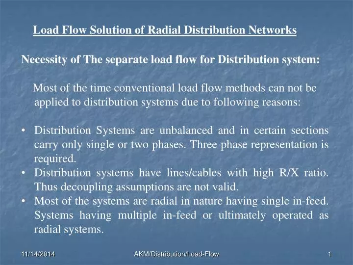
Load Flow Solution of Radial Distribution Networks. Necessity of The separate load flow for Distribution system: Most of the time conventional load flow methods can not be applied to distribution systems due to following reasons:

E N D
Load Flow Solution of Radial Distribution Networks • Necessity of The separate load flow for Distribution system: • Most of the time conventional load flow methods can not be applied to distribution systems due to following reasons: • Distribution Systems are unbalanced and in certain sections carry only single or two phases. Three phase representation is required. • Distribution systems have lines/cables with high R/X ratio. Thus decoupling assumptions are not valid. • Most of the systems are radial in nature having single in-feed. Systems having multiple in-feed or ultimately operated as radial systems. AKM/Distribution/Load-Flow
Backward & Forward Propagation Method • In general all the methods used for a radial system works as backward-forward fashion. • Starts with some assumed voltages at each bus, except the source node. • In the backward propagation, adds all the load currents and downstream branch currents (computed at the assumed voltages) to compute current in the upstream branch. • Starting from the source node, in the forward propagation, updates the bus voltages utilizing the branch currents computed in the backward propagation. • Backward-forward propagation continues till voltages at all the buses converge within pre-specified tolerance. AKM/Distribution/Load-Flow
Methodology-I • A simple and powerful method for load flow solution of radial distribution network. • The method is based on computation of • Bus-Injection to Branch-Current Matrix • Branch-Current to Bus-Voltage Matrix • The BIBC matrix is responsible for the variation between the bus current injection and branch current, • And the BCBV matrix is responsible for the variation between the branch current and bus voltage. Let’s consider an example AKM/Distribution/Load-Flow
From the network an algorithm is developed to compute the nodes fed by a particular branch: • For example network B5 = I6 B3 = I4 + I5 B1 = I2 + I3 +I4 +I5 + I6 Furthermore, the Bus Injection to Branch-Current (BIBC) matrix can be obtained as, AKM/Distribution/Load-Flow
Branch-Current to Bus-Voltage Matrix • The relations between the branch currents and bus voltages is then obtained • For example feeder it can be seen that V2= V1 – B1Z12 V3= V2 – V2 Z23 V4= V3 – B3 Z34 Where Vi is the bus voltage of Bus i, and Zij is the line impedance between Bus i and Bus j. From the above the voltage at each buses can be obtained as a function of bus 1 (substation voltage) For example V4 =V1 – B1Z2 –B2Z23 –B3Z34 AKM/Distribution/Load-Flow
Thus the bus voltages can be updated as • The above expression can be written as [V] = [BCBV] [BIBC][I] = [DLF] [I] AKM/Distribution/Load-Flow
Overall procedure: • Read the system configuration,physical parameters and loads • Compute [BCBV] and [BIBC] Matrices • Assume the voltage at each bus as 1+j0 • Compute the node currents as: Ii(k) =[ (Pi(k) + j Qi(k))/ Vi(k)]* {k is the iteration no.} • Compute [V] = [BCBV] [BIBC][I] and update voltages • Compute the branch real and Reactive loss as: PLj(k)= Bj2Rj and QLj(k)= Bj2Xj {j is the branch no.} • Add these losses to the demand of sending end node of the respective branch (j): Pi(k)= Pi(k-1) + PLj(k) and Qi(k)= Qi(k-1) + QLj(k) • Check V(k)- V(k-1) less than convergence criterion if not go back to step 4 and repeat the whole procedure • Compute total system losses and print node voltages AKM/Distribution/Load-Flow
The Load-flow methodology could be employed either for the individual Feeder or for the whole substationat a time itself. • The Substation transformer could be included in the load flow as a line parameter if reference is to be considered as primary of the sub-station. • It can be observed that the methodology described can be viewed as a special G-S method with S/S as a slack bus and no other generator buses. • The method includes complex variable (trigonometric functions) during analysis making programming bit complex. • The number of iteration though less than G-S method but still large number of iteration required. AKM/Distribution/Load-Flow
Methodology-II • The methods derives the voltage magnitude and phase angle explicitly in terms of real and reactive powers from a node and branch resistance and reactance. • In other word, the methods involves only evaluation of a simple algebraic expression of voltage magnitude and no trigonometric functions are used. • Thus, computationally the methods are very efficient and require less computer memory . • Maximum 4 to 5 iteration will require for convergences for a practical distribution network. AKM/Distribution/Load-Flow