Download
1 / 44
440 likes | 451 Views
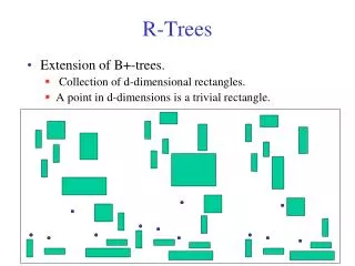
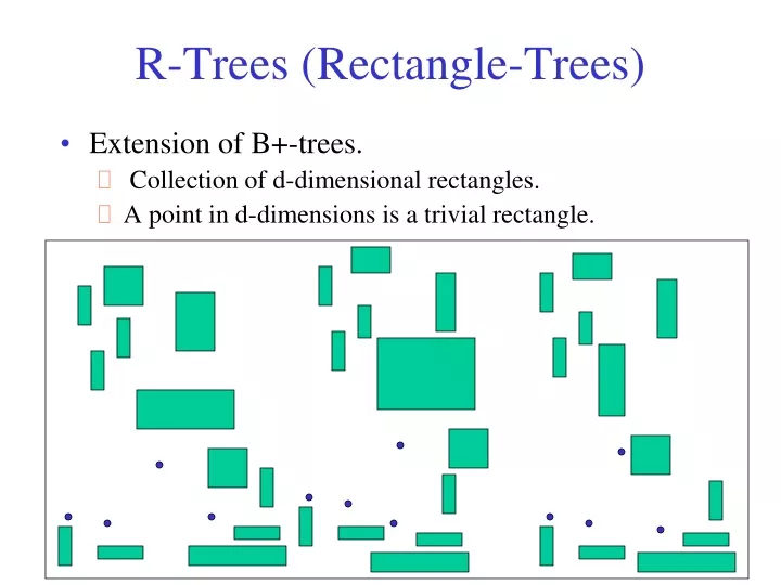
R-Trees (Rectangle-Trees). Extension of B+-trees. Collection of d-dimensional rectangles. A point in d-dimensions is a trivial rectangle. Non-rectangular Data. Non-rectangular data may be represented by minimum bounding rectangles (MBRs). Operations. Insert Delete

E N D
R-Trees (Rectangle-Trees) • Extension of B+-trees. • Collection of d-dimensional rectangles. • A point in d-dimensions is a trivial rectangle.
Non-rectangular Data • Non-rectangular data may be represented by minimum bounding rectangles (MBRs).
Operations • Insert • Delete • Find all rectangles that intersect a query rectangle. • Good for large rectangle collections stored on disk.
R-Trees—Structure • Data nodes (leaves) contain rectangles. • Index nodes (non-leaves) contain MBRs for data in subtrees. • MBR for rectangles or MBRs in a non-root node is stored in parent node.
R-Trees—Structure • R-tree of order M. • Each node other than the root has between m <= ceil(M/2) and M rectangles/MBRs. • Assume m = ceil(M/2) henceforth. • Typically, m = ceil(M/2). • Root has between 2 and M rectangles/MBRs. • Each index node has as many MBRs as children. • All data nodes are at the same level.
Example • R-tree of order 4. • Each node may have up to 4 rectangles/MBRs.
Example • Possible partitioning of our example data into 12 leaves.
m n o p a c d e k l b f g h i j Example • Possible R-tree of order 4 with 12 leaves. Leaves are data nodes that contain 4 input rectangles each. a-p are MBRs
m n o p a c d e k l b f g h i j m Example • Possible corresponding grouping. a b c d
m n o p a c d e k l b f g h i j n m Example • Possible corresponding grouping. e f a b c d
m n o p a c d e k l b f g h i j n m o p Example • Possible corresponding grouping. e f a b g h c d i
Query • Report all rectangles that intersect a given rectangle.
Query • Start at root and find all MBRs that overlap query. • Search corresponding subtrees recursively.
m n o p a c d e k l b f g h i j n m o p Query a x a a
m n o p a c d e k l b f g h i j n a m b o p c d Query • Search m. a a x x
Insert • Similar to insertion into B+-tree but may insert into any leaf; leaf splits in case capacity exceeded. • Which leaf to insert into? • How to split a node?
n m o p Insert—Leaf Selection • Follow a path from root to leaf. • At each node move into subtree whose MBR area increases least with addition of new rectangle.
Insert—Leaf Selection • Insert into m. m
Insert—Leaf Selection • Insert into n. n
Insert—Leaf Selection • Insert into o. o
Insert—Leaf Selection • Insert into p. p
M = 8, m = 4 Insert—Split A Node • Split set of M+1 rectangles/MBRs into 2 sets A and B. • A and B each have at least m rectangles/MBRs. • Sum of areas of MBRs of A and B is minimum.
Insert—Split A Node • Split set of M+1 rectangles/MBRs into 2 sets A and B. • A and B each have at least m rectangles/MBRs. • Sum of areas of MBRs of A and B is minimum. M = 8, m = 4
Insert—Split A Node • Split set of M+1 rectangles/MBRs into 2 sets A and B. • A and B each have at least m rectangles/MBRs. • Sum of areas of MBRs of A and B is minimum. M = 8, m = 4
(M+1)! m!(M+1-m)! Insert—Split A Node • Exhaustive search for best A and B. • Compute area(MBR(A)) + area(MBR(B)) for each possible A. • Note—for each A, the B is unique. • Select partition that minimizes this sum. • When |A| = m = ceil(M/2), number of choices for A is Impractical for large M.
Insert—Split A Node • Grow A and B using a clustering strategy. • Start with a seed rectangle a for A and b for B. • Grow A and B one rectangle at a time. • Stop when the M+1 rectangles have been partitioned into A and B.
M = 8, m = 4 Insert—Split A Node • Quadratic Method—seed selection. • Let S be the set of M+1 rectangles to be partitioned. • Find a and b inS that maximize area(MBR(a,b)) – area(a) – area(b)
M = 8, m = 4 Insert—Split A Node • Quadratic Method—seed selection. • Let S be the set of M+1 rectangles to be partitioned. • Find a and b inS that maximize area(MBR(a,b)) – area(a) – area(b)
M = 8, m = 4 Insert—Split A Node • Quadratic Method—assign remaining rectangles/MBRs. • Find an unassigned rectangle c that maximizes |area(MBR(A,c)) – area(MBR(A)) - (area(MBR(B,c)) – area(MBR(B)))|
M = 8, m = 4 Insert—Split A Node • Quadratic Method—assign remaining rectangles/MBRs. • Find an unassigned rectangle c that maximizes |area(MBR(A,c)) – area(MBR(A)) - (area(MBR(B,c)) – area(MBR(B)))|
M = 8, m = 4 Insert—Split A Node • Quadratic Method—assign remaining rectangles/MBRs. • Assign c to partition whose area increases least.
M = 8, m = 4 Insert—Split A Node • Quadratic Method—assign remaining rectangles/MBRs. • Continue assigning in this way until all remaining rectangles must necessarily be assigned to one of the two partitions for that partition to have m rectangles.
M = 8, m = 4 Insert—Split A Node • Linear Method—seed selection. • Choose a and b to have maximum normalized separation.
M = 8, m = 4 Insert—Split A Node • Linear Method—seed selection. • Choose a and b to have maximum normalized separation. Separation in x-dimension larger left – smaller right
Insert—Split A Node • Linear Method—seed selection. • Choose a and b to have maximum normalized separation. M = 8, m = 4 Rectangles with max x-separation largest left – smallest right
Insert—Split A Node • Linear Method—seed selection. • Choose a and b to have maximum normalized separation. M = 8, m = 4 Divide by x-width to normalize
M = 8, m = 4 Insert—Split A Node • Linear Method—seed selection. • Choose a and b to have maximum normalized separation. Separation in y-dimension larger bottom – smaller top
Insert—Split A Node • Linear Method—seed selection. • Choose a and b to have maximum normalized separation. M = 8, m = 4 Rectangles with max y-separation largest bottom – smallest top
Insert—Split A Node • Linear Method—seed selection. • Choose a and b to have maximum normalized separation. M = 8, m = 4 Divide by y-width to normalize
Insert—Split A Node • Linear Method—assign remainder. • Assign remaining rectangles in random order. • Rectangle is assigned to partition whose MBR area increases least. • Stop when all remaining rectangles must be assigned to one of the partitions so that the partition has its minimum required m rectangles. M = 8, m = 4
Delete • If leaf doesn’t become deficient, simply readjust MBRs in path from root. • If leaf becomes deficient, get from nearest sibling (if possible) and readjust MBRs. • Combine with sibling as in B+ tree. • Could instead do a more global reorganization to get better R-tree.
Variants • R*-tree • Leaf selection and node overflows in insertion handled differently. • Hilbert R-tree
Related Structures • R+-tree • Index nodes have non-overlapping rectangles. • A data object may be represented in several data nodes. • No upper bound on size of a data node. • No bounds (lower/upper) on degree of an index node.
Related Structures • Cell tree • Combines BSP and R+-tree concepts. • Index nodes have non-overlapping convex polyhedrons. • No lower/upper bound on size of a data node. • Lower bound (but not upper) on degree of an index node.