Download

1 / 29
340 likes | 607 Views
R-Trees. Accessing Spatial Data. In the beginning…. The B-Tree provided a foundation for R-Trees. But what’s a B-Tree? A data structure for storing sorted data with amortized run times for insertion and deletion

E N D
R-Trees Accessing Spatial Data
In the beginning… • The B-Tree provided a foundation for R-Trees. But what’s a B-Tree? • A data structure for storing sorted data with amortized run times for insertion and deletion • Often used for data stored on long latency I/O (filesystems and DBs) because child nodes can be accessed together (since they are in order)
B-Tree From wikipedia
What’s wrong with B-Trees • B-Trees cannot store new types of data • Specifically people wanted to store geometrical data and multi-dimensional data • The R-Tree provided a way to do that (thanx to Guttman ‘84)
R-Trees • R-Trees can organize any-dimensional data by representing the data by a minimum bounding box. • Each node bounds it’s children. A node can have many objects in it • The leaves point to the actual objects (stored on disk probably) • The height is always log n (it is height balanced)
R-Tree Example From http://lacot.org/public/enst/bda/img/schema1.gif
Operations • Searching: look at all nodes that intersect, then recurse into those nodes. Many paths may lead nowhere • Insertion: Locate place to insert node through searching and insert. • If a node is full, then a split needs to be done • Deletion: node becomes underfull. Reinsert other nodes to maintain balance.
Splitting Full Nodes • Linear – choose far apart nodes as ends. Randomly choose nodes and assign them so that they require the smallest MBR enlargement • Quadratic – choose two nodes so the dead space between them is maximized. Insert nodes so area enlargement is minimized • Exponential – search all possible groupings • Note: Only criteria is MBR area enlargement
Demo • How can we visualize the R-Tree • By clicking here
Variants - R+ Trees • Avoids multiple paths during searching. • Objects may be stored in multiple nodes • MBRs of nodes at same tree level do not overlap • On insertion/deletion the tree may change downward or upward in order to maintain the structure
R+ Tree http://perso.enst.fr/~saglio/bdas/EPFL0525/sld041.htm
Variants: Hilbert R-Tree • Similar to other R-Trees except that the Hilbert value of its rectangle centroid is calculated. • That key is used to guide the insertion • On an overflow, evenly divide between two nodes • Experiments has shown that this scheme significantly improves performance and decreases insertion complexity. • Hilbert R-tree achieves up to 28% saving in the number of pages touched compared to R*-tree.
Hilbert Value?? • The Hilbertvalue of an object is found by interleaving the bits of its x and y coordinates, and then chopping the binary string into 2-bit strings. • Then, for every 2-bit string, if the value is 0, we replace every 1 in the original string with a 3, and vice-versa. • If the value of the 2-bit string is 3, we replace all 2’s and 0’s in a similar fashion. • After this is done, you put all the 2-bit strings back together and compute the decimal value of the binary string; • This is the Hilbertvalue of the object. http://www-users.cs.umn.edu/research/shashi-group/CS8715/exercise_ans.doc
R*-Tree • The original R-Tree only uses minimized MBR area to determine node splitting. • There are other factors to consider as well that can have a great impact depending on the data • By considering the other factors, R*-Trees become faster for spatial and point access queries.
Problems in original R-Tree • Because the only criteria is to minimize area • Certain types of data may create small areas but large distances which will initiate a bad split. • If one group reaches a maximum number of entries, the rest of assigned without consideration of their geometry. • Greene tried to solve, but he only used the “split axis” – more criteria needs to be used
Splitting overfilled nodes Why is this overfull?
R*-Tree Parameters • Area covered by a rectangle should be minimized • Overlap should be minimized • The sum of the lengths of the edges (margins) should be minimized • Storage utilization should be maximized (resulting in smaller tree height)
Splitting in R*-Trees • Entries are sorted by their lower value, then their upper value of their rectangles. All possible distributions are determined • Compute the sum of the margin values and choose the axis with the minimum as the split axis • Along the split axis, choose the distribution with the minimum overlap • Distribute entries into these two groups
Deleting and Forced Re-insertion • Experimentally, it was shown that re-inserting data provided large (20-50%) improvement in performance. • Thus, randomly deleting half the data and re-inserting is a good way to keep the structure balanced.
Results • Lots of data sets and lots of query types. • One example: Real Data: MBRs of elevation lines. 100K objects Disk accesses On insert Query Storage util. After build up
RC-Trees • Changing motivations: • Memory large enough to store objects • It’s possible to store the object geometry and not just the MBR representation. • Data is dynamic and transient • Spatial objects naturally overlap (ie: stock market triggers)
RC-Trees • Take advantage of dynamic segmentation • If the original geometry is thrown away, then later on the MBR cannot be modified to represent new changes to the tree • RC Tree does • Clipping • Domain Reduction • Rebalancing
Discriminators • A discriminator is used to decide (in binary) which direction a node should go in. (It means it’s a binary tree, unlike other R-Trees) • It partitions the space • If an object intersects a discriminator, the object can be clipped into two parts • When an object is clipped, the space it takes up (in terms of its MBR) is reduced (aka domain reduction) • This allows for removal of dead space and faster point query lookups
Operations • Insert, Delete and Search are straightforward • What happens on an node that has been overflowed? • Choose a discriminator to partition the object into balanced sets • How is a discriminator chosen?
Partitioning • Two methods for finding a discriminator for a partition • RC-MID – faster, but ignores balancing and clipping. Uses pre-computed data to determine and average discriminator. • Problems? • Different distributions greatly affect partition • Space requirements can be huge
Partitioning Take 2 • RC-SWEEP • sorts objects. • Candidates for discriminators are the boundaries of the MBRs • Assign a weight to each candidate using a formula not shown here • Choose the minimum • Problems? • Slower, but space costs much better than RC-MID (which keeps info about nodes)
Rebuilding • The tree can take a certain degree of flexibility in its structure before needing to be rebalanced • On an insert, check if the height is too imbalanced • If so, go to the imbalanced subtree and flush the items, sort and call split on them to get a better balancing
Experimentation • CPU execution time not a good measure. (although they still calculate it) • Instead use number of discriminators compared • Lots of results • Result summary: • Insertion a little more expensive (because of possible rebalancing) • Querying for point or spatial data faster (and fewer memory accesses) than all previous incarnations • Storage requirements not that bad • Dynamic segmentation (ie recalculating MBRs) can help a lot • Controlling space with “γ” factor (by disallowing further splitting) controls space costs