Download
1 / 19
190 likes | 298 Views
EEE422 Signals and Systems Laboratory. Filters (FIR) Kevin D. Donohue Electrical and Computer Engineering University of Kentucky. Filters. Filter are designed based on specifications given by: spectral magnitude emphasis delay and phase properties through the group delay and phase spectrum

E N D
EEE422 Signals and Systems Laboratory Filters (FIR) Kevin D. DonohueElectrical and Computer EngineeringUniversity of Kentucky
Filters Filter are designed based on specifications given by: • spectral magnitude emphasis • delay and phase properties through the group delay and phase spectrum • implementation and computational structures Filter implementations are broadly classified based on the extent of their impulse responses: • FIR = finite impulse response (impulse response goes to zero and stays there after a finite number of time samples) • IIR = infinite impulse response (impulse response continues infinitely in time).
Filter Specifications Example:Low-pass filter frequency response
Filter Specifications Example Low-pass filter frequency response (in dB)
Filter Specifications Example Low-pass filter frequency response (in dB) with ripple in both bands
Useful Filter Functions The sinc function and the rectangular pulse form a Fourier transform pair.
Ideal Low-Pass Filter Response indicates the ideal low-pass filter is non-causal and infinite. If using in a filter design process need to approximate
Impulse Response Method for FIR Filter Design Approach: • Create ideal filter specifications for the magnitude response. • Generate impulse response through sinc function relationship. • Shift (delay) in time so sufficient response energy occurs after t=0 to make response closer to ideal in a causal implementation • Truncate sequence to make causal and finite: include 0 to N-1 to obtain coefficients for an Nth order filter. A tapering window is used to limit sharp transitions at the end points, which translate into ripple in the pass and stop bands.
Example Use impulse response method to compute a 24th order low-pass filter for fs = 1 and cut-off frequency of .125 Hz.
Example Use impulse response method to compute a 24th order low-pass filter for fs= 1 and cut-off frequency of .125 Hz. t = [24/2:1:24/2]; % evaluate since at 25 symmetric time pointsbtemp = 0.25*sinc(0.25*t)
Example Delay response by 24/2 = 12 seconds. Then apply tapering window: wtap = hamming(25); plot(t+12,wtap,’g—’)
Example Plot below are the coefficient values used to implement the FIR filter. Because is symmetric it will have a linear phase that accounts for the shift in time. All filtered outputs will undergo a 24/2 sample delay.
Example Use fir1() Generate filter coefficient and check response by examining the Magnitude and Phase response. fs = 1; % Sampling Frequency b = fir1(24,.125/(fs/2), hamming(25)); % Compute filter coefficients, normalize frequency by Nyquest [h,f] = freqz(b,1,1024,1); % Arguments: b is vector of FIR coefficients, 1 is the scaling on the output term, 1024 are number of points to evaluate frequency response at, 1 is the sampling frequency plot(f,abs(h)) plot(f,phase(h))
Example Use fir1() Generate filter coefficients without a tapering window and plot magnitude and phase response: fs = 1; % Sampling Frequency b = fir1(24,.125/(fs/2), boxcar(25)); % Compute filter coefficients, normalize frequency by Nyquest [h,f] = freqz(b,1,1024,1); % Arguments: b is vector of FIR coefficients, 1 is the scaling on the output term, 1024 are number of points to evaluate frequency response at, 1 is the sampling frequency plot(f,abs(h)) plot(f,phase(h))
Parks-Mcclellan Filter To better control ripple over designated pass and stop bands, an iterative algorithm was applied to adjust filter coefficients to spread the ripple out making it uniform over the bands of interest, thus minimizing the maximum deviation from the ideal flat pass/stop band for a given order.
Parks-Mcclellan Filter Example Need to specify band range and amplitude over normalized frequency range. Can use as many bands as desired, but there should be space between defined bands for a transition to occur. Example: apply previous design specs for PM filter fs = 1 % Sampling Frequency f = [0 .12 .13 .5]/(fs/2) % Need to normalize at Nyquest mag = [1 1 0 0]; % define pass and stopband amplitudes corresponding to vector f bpm = firpm(24, f,mag); % create FIR filter coefficients Interval between pass and stop band – transition band include specified cut-off (.125 Hz)
PM Filter Results Examine magnitude and phase response of resulting filter:
Parks-Mcclellan Filter Example Try again with bigger transition band fs = 1 % Sampling Frequency f = [0 .10 .15 .5]/(fs/2) % Need to normalize at Nyquest mag = [1 1 0 0]; % define pass and stopband amplitudes corresponding to vector f bpm = firpm(24, f,mag); % create FIR filter coefficients Interval between pass and stop band – transition band include specified cut-off (.125 Hz)
PM Filter Results Examine and compare magnitude and phase responses of resulting filters: