Download
1 / 21
240 likes | 637 Views
Signals and Systems. Outline. Signals Continuous-time vs. discrete-time Analog vs. digital Unit impulse Continuous-Time System Properties Sampling Discrete-Time System Properties Conclusion. Review. Many Faces of Signals.

E N D
Outline • Signals Continuous-time vs. discrete-time Analog vs. digital Unit impulse • Continuous-Time System Properties • Sampling • Discrete-Time System Properties • Conclusion
Review Many Faces of Signals • Function, e.g. cos(t) in continuous time orcos(p n) in discrete time, useful in analysis • Sequence of numbers, e.g. {1,2,3,2,1} or a sampled triangle function, useful in simulation • Set of properties, e.g. even and causal,useful in reasoning about behavior • A piecewise representation, e.g.useful in analysis • A generalized function, e.g. d(t),useful in analysis
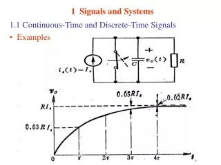
Review Continuous-Time vs. Discrete-Time • Continuous-time signals can be modeled as functions of a real argument x(t) where time, t, can take any real value x(t) may be 0 for a given range of values of t • Discrete-time signals can be modeled as functions of argument that takes values from a discrete set x[n] where n {...-3,-2,-1,0,1,2,3...} Integer time index, e.g. n, for discrete-time systems • Values for x may be real-valued or complex-valued
1 -1 Review Analog vs. Digital • Amplitude of analog signal can take any real or complex value at each time/sample • Amplitude of digital signal takes values from a discrete set
-e e t -e e t Review Unit Impulse • Mathematical idealism foran instantaneous event • Dirac delta as generalizedfunction (a.k.a. functional) • Selected properties Unit area: Sifting providedg(t) is defined att = 0 Scaling: • We will leave (0) undefined Unit Area Unit Area
(1) Unit Area t 0 Unit Impulse • We will leave (0) undefined Some signals and systems textbooks assign d(0) = ∞ • Plot Dirac delta as arrow at origin Undefined amplitude at origin Denote area at origin as (area) Height of arrow is irrelevant Direction of arrow indicates sign of area • With d(t) = 0 for t 0, it is tempting to think f(t) d(t) = f(0) d(t) f(t) d(t-T) = f(T) d(t-T) Simplify unit impulse under integration only No!
Simplifying d(t) under integration Assuming (t) is defined at t=0 What about? What about? By substitution of variables, Other examples What about at origin? Review Unit Impulse Before Impulse After Impulse
Unit Impulse • Relationship between unit impulse and unit step • What happens at the origin for u(t)? u(0-) = 0 and u(0+) = 1, but u(0) can take any value Common values for u(0) are 0, ½, and 1 u(0) = ½ is used in impulse invariance filter design: L. B. Jackson, “A correction to impulse invariance,” IEEE Signal Processing Letters, vol. 7, no. 10, Oct. 2000, pp. 273-275.
x(t) x[n] T{•} T{•} y(t) y[n] Review Systems • Systems operate on signals to produce new signals or new signal representations • Continuous-time system examples y(t) = ½ x(t) + ½ x(t-1) y(t) = x2(t) • Discrete-time system examples y[n] = ½ x[n] + ½ x[n-1] y[n] = x2[n] Squaring function can be used in sinusoidal demodulation Average of current input and delayed input is a simple filter
Review Continuous-Time System Properties • Let x(t), x1(t), and x2(t) be inputs to a continuous-time linear system and let y(t), y1(t), and y2(t) be their corresponding outputs • A linear system satisfies Additivity: x1(t) + x2(t) y1(t) + y2(t) Homogeneity: a x(t) a y(t) for any real/complex constant a • For time-invariant system, shift of input signal by any real-valued t causes same shift in output signal, i.e. x(t - t) y(t - t), for all t • Example: Squaring block Quick test to identify some nonlinear systems? x(t) ()2 y(t)
y(t) x(t) Role of Initial Conditions • Observe a system starting at time t0 Often use t0 = 0 without loss of generality • Integrator • Integrator observed for t t0 Linear system if initial conditions are zero (C0 = 0) Time-invariant system if initial conditions are zero (C0 = 0) C0 is due to initial conditions y(t) x(t)
y(t) x(t) x(t) y(t) x(t) y(t) Review Continuous-Time System Properties • Ideal delay by T seconds. Linear? • Scale by a constant (a.k.a. gain block) Two different ways to express it in a block diagram Linear? Time-invariant? Role of initial conditions?
… … S Continuous-Time System Properties • Tapped delay line Linear? Time-invariant? Each T represents a delay of T time units There are M-1 delays Coefficients (or taps) are a0, a1, …aM-1 Role of initial conditions?
Continuous-Time System Properties • Amplitude Modulation (AM) y(t) = Ax(t) cos(2p fc t) fc is the carrierfrequency(frequency ofradio station) A is a constant Linear? Time-invariant? • AM modulation is AM radio if x(t) = 1 + kam(t) where m(t) is message (audio) to be broadcastand | kam(t)| < 1 (see lecture 19 for more info) y(t) x(t) A cos(2 p fc t)
n s(t) Ts t Ts Sampled analog waveform Review Generating Discrete-Time Signals • Many signals originate in continuous time Example: Talking on cell phone • Sample continuous-time signalat equally-spaced points in timeto obtain a sequence of numbers s[n] = s(n Ts) for n {…, -1, 0, 1, …} How to choose sampling period Ts? • Using a formula x[n] = n2 – 5n + 3 on right for 0 ≤ n ≤ 5 How does x[n] look in continuous time?
Review Discrete-Time System Properties • Let x[n], x1[n] and x2[n] be inputs to a linear system • Let y[n], y1[n] and y2[n] be corresponding outputs • A linear system satisfies Additivity: x1[n] + x2[n] y1[n] + y2[n] Homogeneity: a x[n] a y[n] for any real/complex constant a • For a time-invariant system, a shift of input signal by any integer-valued m causes same shift in output signal, i.e. x[n - m] y[n - m], for all m • Role of initial conditions?
… … S Discrete-Time System Properties • Tapped delay line in discrete time • Linear? Time-invariant? See also slide 5-4 Each z-1 represents a delay of 1 sample There are M-1 delays Coefficients (or taps) are a0, a1, …aM-1 Role of initial conditions?
d[n] 1 n -3 -2 -1 1 2 3 d[n] h[n] Discrete-Time System Properties • Let d[n] be a discrete-time impulse function, a.k.a. Kronecker delta function: • Impulse response is response of discrete-time LTI system to discrete impulse function Example: delay by one sample • Finite impulse response filter Non-zero extent of impulse response is finite Can be in continuous time or discrete time Also called tapped delay line (slides 3-14, 3-18, 5-4)
Continuous time Linear? Time-invariant? Discrete time Linear? Time-invariant? f(t) y(t) f[n] y[n] Discrete-Time System Properties See also slide 5-18
Conclusion • Continuous-time versus discrete-time:discrete means quantized in time • Analog versus digital:digital means quantized in amplitude • Digital signal processor Discrete-time and digital system Well-suited for implementing LTI digital filters • Example of discrete-time analog system? • Example of continuous-time digital system?