Download
1 / 65
650 likes | 653 Views
This paper explores the importance of constraints in system identification, including incorporating prior knowledge, avoiding trivial solutions, mitigating bias, and imposing stability and structures. It discusses different estimation approaches and their relationship to constraints.

E N D
On the Role of Constraints in System Identification Arie Yeredor Dept. of Electrical Engineering - Systems School of Electrical Engineering Tel-Aviv University
Outline • System identification – problem models • Estimation and approximation approaches • The role(s) of constraints: • Incorporating prior knowledge • Avoiding trivial solutions • Mitigating bias • Imposing stability • Imposing structures • Conclusion
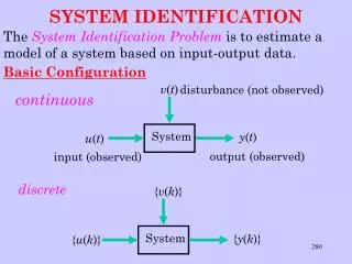
System Identification • The single-input single-output (SISO) linear, time-invariant, causal, stable model(with output-noise only): • It is desired to estimate from observations of the noisy output and possibly the input .
System Identification (contd.) • In the general case, this involves estimation of an infinite number of parameters . • Often the system is parameterized as a rational system of general order : thereby giving rise to the following causal difference equation:
System Identification (contd.) • With this parameterized representation it is desired to estimate the parameters
System Identification (contd.) • The same difference equation also admits a state-space representation as follows: Defining a state-vector and a “driving vector” , we can express the same relation usingnote that this representation is not unique.
System Identification (contd.) • With this parameterized representation it is desired to estimate the matrices(with tolerable ambiguities, as long as the implied input-output relation is maintained).
System Identification (contd.) • For Multiple-Inputs Multiple Outputs (MIMO) systems, similar difference equations or state-space equations can be obtained:or:
Estimation approaches • The Maximum Likelihood (ML) approach is often guaranteed to provide consistent estimates of the parameters, and, moreover, is asymptotically optimal (in the sense of minimum mean square error, among all (asymptotically) unbiased estimates). • ML estimation involves maximization of the Likelihood function with respect to the parameters, and no “artificial” constraints are required (except for the purpose of incorporating prior knowledge, if available). • However, in the rational model with noisy output measurements ML estimation can become computationally unattractive.
Estimation approaches (contd) • It is therefore often tempting to resort to “heuristic” Least-Squares (LS)-driven approaches, such as Errors-In-Variables or subspace-based approaches. • In these contexts, the free parameters often have to be constrained, and mis-constraining may result in inconsistent estimates.
A “Toy-Example” • Consider the first-order autoregressive (AR(1)) process • is the (noiseless) output of the systemwhose input is the (unobserved) process , known to be zero-mean, white with variance .
“Toy-example” (contd.) • Assuming that is Gaussian, the ML estimate seeks so as to maximize the likelihood, given by
“Toy-example” (contd.) Where . An equivalent constrained minimization problem iswhose solution is ,which is a consistent estimate of .
“Toy-example” (contd.) • What if we wanted to minimize the same LS criterion, subject to a different, quadratic constraint (and then “impose” by scaling)? • The solution is the eigenvector of corresponding to the smallest eigenvalue.This is either or(depending on the sign of ).Therefore, following normalization we would always get , which is always inconsistent.
“Toy-example” (contd.) • Of course, it can now be argued that the quadratic constraint is inappropriate for the problem. But what if it were? • Consider the slightly different model equationwhere it is now known that(e.g., if it is known thatfor some unknown ).
“Toy-example” (contd.) • The quadratic constraint inis now “appropriate” for the problem, but the minimization would still yield the useless, inconsistent estimate ! • However, if we were to use the “inappropriate” linear constraint (and then normalize), we would get a consistent estimate again!
“Toy-example” (contd.) • This is because in the second problem (with the quadratic constraint), the “heuristic” LS criterion is no longer ML, and therefore its consistency is not guaranteed, but rather depends on the constraint. The consistent ML criterion for this problem is . • Note that no constraints are necessary here for avoiding the “trivial” solution . However, any relevant constraints may be incorporated. • Note that with the linear (monic) constraint, the ML criterion is reduced to the LS criterion.
“Toy-example”: conclusion • When a “heuristic” LS criterion is used, using the “wrong” constraints (even if they are consistent with the problem at hand) may result in inconsistent, or even useless estimates.
General formulation • Any cost-function-based estimation scheme (e.g., ML, LS-based) would generally be cast as a constrained minimization problem,where are the observations, are the parameters of interest and are possible auxiliary “nuisance parameters”. • The constraints (vector-)function may effectively constrain , or both.
The role of constraints • Constraints on either the parameters of interest or the nuisance parameters (mainly required for LS-driven, non-ML criteria) can emerge from various perspectives or requirements.Some possible motivations are: • Avoiding trivial solutions • Mitigating bias • Incorporating prior knowledge • Imposing stability • Imposing structures
LS-based criteria • A popular LS criterion, associated with the difference equation model, is the following. Recall the SISO model equation,
LS-based criteria (contd.) which can also be written in matrix form as
LS-based criteria (contd.) • In the case of an exact model and noiseless observations, equations are sufficient for exact identification of the system parameters. • In the presence of model inaccuracies, more equations can be used in order to obtain an ordinary LS solution. • However, in the presence of output (and / or input) noise, different approaches can be taken.
The TLS approach • When the true output is replaced by the noisy output , the matrix equation can be reformulated as follows:
The TLS approach (contd.) • The (weighted) TLS approach then seeks a minimal perturbation of the “output section” of the data matrix, such that the equation is satisfied with some . • A “natural” (linear) constraint on for avoiding the trivial solution is . • Note that the formulation here involves another set of “nuisance parameters” , which are the required perturbation matrix’ elements. Note that in this framework, the nuisance parameters are unconstrained.
The TLS approach (contd.) • The TLS constrained minimization can therefore be formulated as(where denotes the first column of the identity matrix). • The linear constraint on can be replaced with a quadratic constraint, such as (with almost any nonzero ) with no effect on the resulting solution in this case.
The Equation Error approach • Although the TLS approach attempts to account for the output measurements noise by trying to retrieve some “underlying data”, the resulting estimate is usually inconsistent. • A possible remedy, which regains consistency by essentially applying the ML estimate (for Gaussian output noise), is the Structured TLS (STLS, De Moor ’94, Markovsky et al., ’05), to which we shall return later. • Somewhat surprisingly, however, it is possible to obtain consistent estimates without accounting for the output noise (as long as it is white), by slightly reformulating the criterion and changing the constraint on (Regalia, ’95).
Equation Error approach (contd.) • Recall the model equation with the true output replaced by the noisy output:Now, rather than modify so as to obtain exact equality, find that minimizes the norm of the left-hand side. • To avoid the trivial solution, has to be constrained.
Equation Error approach (contd.) • The resulting criterion becomes wherewhere are columns of (resp.)
Equation Error approach (contd.) • Under weak ergodicity conditions on and , the empirical correlations tend asymptotically to the true correlations. • Thus, to study the estimator’s consistency, we substitute the true correlations into the criterion,where the first transition is due to the assumption that the observation noise is uncorrelated with the input, and is the same LS criterion, evaluated with the true (noiseless) output data.
Equation Error approach (contd.) • It is therefore evident, that the noisy output criterion only differs (asymptotically) from the noiseless output criterion by the term . • Under the assumption of white output noise (with ), a quadratic constraint on of the form would render the noisy criterion identical to the noiseless criterion up to an additive constant. • Since the noiseless criterion is minimized by the true , that value would also minimize the noisy criterion (properly constrained), regaining consistency and eliminating the bias. • This will not happen if the linear constraint is used – which would result in severe bias.
Equation Error approach (contd.) • We demonstrate this concept in the identification of a first-order system, so as to be able to use a two-dimensional plot. We used . • We plot the residual asymptotic cost function following minimization with respect to , vs. all values of . • Values estimated with the linear and quadratic constraints are demonstrated for different noise levels.
Equation Error approach (conclusion) • Therefore, the same criterion with a different constraint, although not a “natural” constraint, turns an inconsistent estimate into a consistent one. • Note that if the noise is not white, but has a known covariance , then the quadratic constraint may be adjusted accordingly, , to maintain consistency.
Incorporating prior knowledge • Quite often, some prior knowledge is available regarding characteristics of the estimated system. • Such information can be incorporated in a Bayesian (or some heuristic approach) when subject to uncertainty. • Otherwise, however, it is desirable to incorporate the prior knowledge in the form of constraints on the estimated parameter, thereby effectively reducing dimensionality and improving accuracy.
Prior knowledge (contd.) • Assume that the system is known to have specific gains at certain frequencies. • At each such frequency: • Either the exact complex-valued gainis known; • Or the magnitude-square gain is known (often more common).