Download
1 / 27
270 likes | 585 Views
Factorial BG ANOVA. Psy 420 Ainsworth. Topics in Factorial Designs. Factorial? Crossing and Nesting Assumptions Analysis Traditional and Regression Approaches Main Effects of IVs Interactions among IVs Higher order designs “Dangling control group” factorial designs

E N D
Factorial BG ANOVA Psy 420 Ainsworth
Topics in Factorial Designs • Factorial? • Crossing and Nesting • Assumptions • Analysis • Traditional and Regression Approaches • Main Effects of IVs • Interactions among IVs • Higher order designs • “Dangling control group” factorial designs • Specific Comparisons • Main Effects • Simple Effects • Interaction Contrasts • Effect Size estimates • Power and Sample Size
Factorial? • Factorial – means that all levels of one IV are completely crossed with all level of the other IV(s). • Crossed – all levels of one variable occur in combination with all levels of the other variable(s) • Nested – levels of one variable appear at different levels of the other variable(s)
Factorial? • Crossing example • Every level of teaching method is found together with every level of book • You would have a different randomly selected and randomly assigned group of subjects in each cell • Technically this means that subjects are nested within cells
Factorial? • Crossing Example 2 – repeated measures • In repeated measures designs subjects cross the levels of the IV
Factorial? • Nesting Example • This example shows testing of classes that are pre-existing; no random selection or assignment • In this case classes are nested within each cell which means that the interaction is confounded with class
Assumptions • Normality of Sampling distribution of means • Applies to the individual cells • 20+ DFs for error and assumption met • Homogeneity of Variance • Same assumption as one-way; applies to cells • In order to use ANOVA you need to assume that all cells are from the same population
Assumptions • Independence of errors • Thinking in terms of regression; an error associated with one score is independent of other scores, etc. • Absence of outliers • Relates back to normality and assuming a common population
Equations • Extension of the GLM to two IVs • = deviation of a score, Y, around the grand mean, , caused by IV A (Main effect of A) • = deviation of scores caused by IV B (Main effect of B) • = deviation of scores caused by the interaction of A and B (Interaction of AB), above and beyond the main effects
Equations • Performing a factorial analysis essentially does the job of three analyses in one • Two one-way ANOVAs, one for each main effect • And a test of the interaction • Interaction – the effect of one IV depends on the level of another IV • e.g. The T and F book works better with a combo of media and lecture, while the K and W book works better with just lecture
Equations • The between groups sums of squares from previous is further broken down; • Before SSbg = SSeffect • Now SSbg = SSA + SSB + SSAB • In a two IV factorial design A, B and AxB all differentiate between groups, therefore they all add to the SSbg
Equations • Total variability = (variability of A around GM) + (variability of B around GM) + (variability of each group mean {AxB} around GM) + (variability of each person’s score around their group mean) • SSTotal = SSA + SSB + SSAB + SSS/AB
Equations • Degrees of Freedom • dfeffect = #groupseffect – 1 • dfAB = (a – 1)(b – 1) • dfs/AB = ab(s – 1) = abs – ab = abn – ab = N – ab • dftotal = N – 1 = a – 1 + b – 1 + (a – 1)(b – 1) + N – ab
Equations • Breakdown of sums of squares
Equations • Breakdown of degrees of freedom
Equations • Mean square • The mean squares are calculated the same • SS/df = MS • You just have more of them, MSA, MSB, MSAB, and MSS/AB • This expands when you have more IVs • One for each main effect, one for each interaction (two-way, three-way, etc.)
Equations • F-test • Each effect and interaction is a separate F-test • Calculated the same way: MSeffect/MSS/AB since MSS/AB is our variance estimate • You look up a separate Fcrit for each test using the dfeffect, dfS/AB and tabled values
Sample data • Sample info • So we have 3 subjects per cell • A has 3 levels, B has 3 levels • So this is a 3 x 3 design
Analysis – Computational • Marginal Totals – we look in the margins of a data set when computing main effects • Cell totals – we look at the cell totals when computing interactions • In order to use the computational formulas we need to compute both marginal and cell totals
Sample data reconfigured into cell and marginal totals Analysis – Computational
Analysis – Computational • Formulas for SS
Analysis – Computational • Example
Analysis – Computational • Example
Analysis – Computational • Example
Analysis – Computational • Example
Analysis – Computational • Fcrit(2,18)=3.55 • Fcrit(4,18)=2.93 • Since 15.25 > 3.55, the effect for profession is significant • Since 14.55 > 3.55, the effect for length is significant • Since 23.46 > 2.93, the effect for profession * length is significant