Download
1 / 9
90 likes | 187 Views
Chapter 4 Network Algorithms. Section 4.1 Shortest Paths Colleen Raimondi. a. 5. b. 3. e. 4. 1. 2. 2. 6. d. c. 4. Section 4.1 Shortest Paths. In this chapter we present algorithms for the solution of two important network optimization problems.

E N D
Chapter 4 Network Algorithms Section 4.1 Shortest Paths Colleen Raimondi
a 5 b 3 e 4 1 2 2 6 d c 4 Section 4.1 Shortest Paths In this chapter we present algorithms for the solution of two important network optimization problems. Network: a graph with a positive integer k(e) assigned to each edge e, it will typically represent the “length” of an edge, in units such as miles, or represent “capacity” of an edge, in units such as megawatts or gallons per minute. Note:Edge (a,b) has a “capacity” of 5, so k(a,b)=5.
Section 4.1 Shortest Paths We begin with an algorithm for a relatively simple problem, finding a shortest path in a network from point a to point z. We say a shortest path because, in general, there may be more than one shortest path from a to z. So when we find a shortest path, we must be able to prove it is shortest without explicitly comparing it with all over a-z paths. Although the problem is now starting to sound difficult, there is still a straightforward algorithmic solution.
Section 4.1 Shortest Path Dijkstra’s algorithm Let variable m be a “distance counter.” For increasing values of m, label vertices whose minimal distance from a vertex a is m. The first label of a vertex will be the previous vertex on the shortest path from a to x. The second label of x will be the length of the shortest path from a to x.
Section 4.1 Shortest Path • Shortest Path Algorithm • Set m=1 and label vertex a with (-,0) (the “-” represents a blank). • Check each edge e=(p,q) from some labeled vertex p to some unlabeled vertex q. Suppose p’s labels are [r,d(p)]. If d(p)+k(e)=m, label q with (p,m). • If all vertices are not yet labeled, increment m by one and go to Step 2. Otherwise go to Step 4. If we are only interested in a shortest path to z, then we go to Step 4 when z is labeled. • For any vertex y, a shortest path from a to y has length d(y), the second label of y. Such a path may be found by backtracking from y (using the first labels).
a 5 b 3 e 4 1 2 2 6 d c 4 Section 4.1 Shortest Path We want to find the shortest path from a to c. a(-,0) m=1; m=3; m=5; The shortest path would be a-d-c. e(d,3) c(d,5) d(a,1)
Section 4.1 Shortest Paths Note: The algorithm given previously has one significant inefficiency: if all sums d(p)+k(e) in Step 2 have values of at least m’>m, then the distance counter m should be increased immediately to m’.
f(i,3) f i 2 i(a,1) a 1 2 3 e 6 7 e(f,4) 4 4 d j r 5 1 j(a,4) 2 g 3 6 r(a,6) k g(e,5) 2 h 9 k(j,6) h(g,7) Section 4.1 Example Example 1 Pg. 134 m=1; m=3; m=4; m=5; m=6; m=7 a(-,0) The shortest path is a-i-e-g-h. We want to find a shortest path from point a to point h.
m=2; m=5; m=6; m=7; m=10; m=12; m=14 f(i,10) 10 n 4 i(m,6) i f f m 6 4 m(-,0) 2 6 8 5 e b 6 d 2 j r e(g,10) 4 3 3 12 2 3 5 d(h,12) g j(m,2) 2 k 4 c r(m,5) g(j,7) h 5 6 20 k(j,5) c(d,14) h(k,10) The shortest path is m-j-k-h-d-c. Section 4.1 Class WorkAs seen on page 135 #1 Use the shortest path algorithm to find the shortest path between vertex c and vertex m.