Download
1 / 38
380 likes | 561 Views
CHAPTER 4: NETWORK LAYER. Packet Switching Virtual Circuits Datagrams Network Routers Internet Protocol IPv4 IPv6 Routing Algorithms IP Routing Broadcast and Multicast. NETWORK LAYER RESPONSIBILITIES. Moving Transport segments from their sources to their destinations.

E N D
CHAPTER 4: NETWORK LAYER • Packet Switching • Virtual Circuits • Datagrams • Network Routers • Internet Protocol • IPv4 • IPv6 • Routing Algorithms • IP Routing • Broadcast and Multicast
NETWORK LAYER RESPONSIBILITIES • Moving Transport segments from their sources to their destinations • Breaking segments into manageable units at the source and reassembling them at the destination • Determining paths for packets to take through the network, and ensuring that those paths are followed. CS 447 Chapter 4 Page 79
CIRCUIT SWITCHING In traditional circuit switching, an end-to-end circuit is established and maintained until one of the endstations terminates the connection. CS 447 Chapter 4 Page 80
PROBLEMS WITH CIRCUIT SWITCHING Circuit switching has one great advantage: once established, the circuit is dedicated, i.e., a communication line is completely open until formally terminated. However, this approach has a number of serious problems: • Many networked applications don’t require a dedicated circuit, so reserving a communication line until an endstation formally terminates it can represent a serious waste of resources. • The route originally selected for the circuit may be optimal to begin with, but may prove to be suboptimal as the communication continues. • An entire, end-to-end path must be found and reserved before any communication is allowed between the two endstations; this is definitely not conducive to many modern applications (e.g., Web surfing, videoconferencing). • Transmission errors are propagated all the way to the destination, requiring retransmission across the entire network. CS 447 Chapter 4 Page 81
PACKET SWITCHING In packet switching, the source’s message is broken into manageable “packets” that are transmitted to the destination individually, not necessarily along the same path. CS 447 Chapter 4 Page 82
THE PROS AND CONS OF PACKET SWITCHING Packet switching remedies the principal problems of circuit switching: • Lines aren’t dedicated, so their utilization is higher. • Messages are “packetized”, so line-sharing is reasonably fair. • Routing may be dynamic, i.e., an alternate route may be chosen when traffic patterns change. • The entire route does not have to be chosen prior to sending any data. • Errors aren’t propagated end-to-end. However, packet switching does have its own set of problems: • Switches must be programmed to make sophisticated routing decisions. • Switches must manage memory for queued packets that await forwarding. • Packets must be prefixed with control headers, increasing overhead. • Endstations must deal with missing packets and packets received out of order. • Without a dedicated circuit, transmission times become unpredictable. CS 447 Chapter 4 Page 83
Routes are chosen when the VC is initially set up • All packets must follow the VC route, even if traffic conditions have improved or worsened • Buffer space must be allocated for each VC • A failed router destroys all VCs running through it • VC routing is handled by a table VIRTUAL CIRCUITS Incoming VC # Source Node Outgoing VC # Next Node 1 3 3 8 4 2 Network Node 5 5 Network Node 7 6 VC3 packet 8 1 VC1 packet VC8 packet VC1 packet VC4 packet VC8 packet Network Node VC7 packet VC2 packet VC3 packet VC5 packet Network Node VC6 packet Network Node Node has a VC table that looks something like this: CS 447 Chapter 4 Page 84
DATAGRAMS Network Node Network Node pkt to dest. X pkt to dest. X pkt to dest. X Network Node pkt to dest. X pkt to dest. X Network Node pkt to dest. X Network Node • No route set-up is done • All packets must contain the full source and destination addresses • Each packet is routed independently • A failed router only affects the packets passing through it when the failure occurs • Congestion control is difficult IP uses a datagram approach to packet switching, while Multiprotocol Link Switching (MPLS) uses virtual circuits. CS 447 Chapter 4 Page 85
PACKET SWITCHING COMPARISONS CS 447 Chapter 4 Page 86
INTERNETWORKING Networks can be connected via a variety of devices, operating at various protocol layers. A router works at the Network Layer to direct incoming packets onto networks that bring them closer to their final destination. A bridge works at the Data Link Layer to store and forward frames from one LAN to another. A repeater works at the Physical Layer to regenerate weak signals on a bit-by-bit basis. Finally, a gateway works at the Transport Layer to interconnect subnetworks by keeping track of incoming and outgoing virtual circuits that may use differing transport protocols. CS 447 Chapter 4 Page 87
NETWORK ROUTERS A router is a network node operating at the Network Layer (and lower), with two primary responsibilities: • Running algorithms to decide where to send incoming datagrams. • Forwarding datagrams from its input ports to its output ports. Input Port Switching Fabric Output Port Lookup, Forwarding, Queueing (Network Layer) Datagram Buffering, Queueing (Network Layer) Bit Reception (Physical Layer) Packet Reception (Data Link Layer) Switching Via Crossbar Bit Release (Physical Layer) Packet Release (Data Link Layer) The router’s input port mechanism contains memory holding a lookup table indicating where to forward packets. If the datagram arrival rate exceeds the forwarding rate, then datagrams are queued inside input buffers. The router’s switching fabric forwards the datagrams from the input ports to the correct output ports. The router’s output port mechanism contains memory buffers for holding datagrams that arrive from the fabric faster than the router’s transmission rate. CS 447 Chapter 4 Page 88
CROSSBAR SWITCHES Both circuit switching and packet switching rely heavily on primitive internal routing that usually takes place on a crossbar switch. inputs outputs Each crosspoint in the switch has a transistor connecting a unique input/output pair. When activated, a crosspoint transfers every signal on its input line onto its output line. Multistage space-division switches, use smaller interconnected crossbar switches to inexpensively connect large numbers of input/output pairs. CS 447 Chapter 4 Page 89
INPUT OR OUTPUT BUFFERS? If a router is forced to buffer datagrams due to excessive traffic (either fast arrival rates or slow transmission rates, should it use input buffers (i.e., holding the datagrams before they are routed) or output buffers (i.e., holding the datagrams after they are routed)? Datagram for output port 3 Router Datagram for output port 4 Datagram for output port 3 Datagram for output port 1 Datagram for output port 3 Note that the use of input buffers can result in datagrams being blocked from proceeding to their output ports, even if the output ports are open, a condition known as Head-of-Line Blocking. CS 447 Chapter 4 Page 90
FRAGMENTATION NETWORK packet packet packet frag frag packet frag frag NETWORK packet packet frag frag frag frag frag frag frag frag Different networks have different packet size limitations, based upon their protocols and their system administrators. To accommodate these differences, gateways may have to break packets into smaller fragments in order to get them through a network. Transparent fragmentation involves breaking packets into fragments upon entrance to a network, and recombining the fragments at the exit gateway. This eliminates the negative effects of fragmentation (i.e., header overhead, destination host reassembly) on the rest of the internetwork. Non-transparent fragmentation involves breaking packets into fragments upon entrance to a network, but recombining the fragments only at their final destination. This eliminates the negative effects of transparency (i.e., repeated fragmenting, common exit gateways) on the rest of the internetwork. CS 447 Chapter 4 Page 91
INTERNET PROTOCOL IP was designed for three primary purposes: 1. Define the basic unit of data transfer (i.e., the data format) through any TCP/IP internet. 2. Perform the routing of data through the internet by selecting appropriate paths. 3. Process packets, generate error messages, and discard packets in such a way to ensure “unreliable” packet delivery. CS 447 Chapter 4 Page 92
THE IPv4 HEADER Version HdrLen Service Type Total Length Identification Flags Fragment Offset Time To Live Protocol Header Checksum Source IP Address Destination IP Address Options & Padding (if any) Version HdrLen Service Type Total Length Identification Flags Fragment Offset Time To Live Protocol Header Checksum Source IP Address Destination IP Address Options & Padding (if any) Version:Version of IP used to create the datagram, used by nodes to process it correctly. HdrLen:Length of the header in 32-bit words (because the Options field has no fixed size). Service Type:3-bit Precedence field, & three 1-bit Delay, Throughput, and Reliability flags. Total Length:Length of the entire datagram in bytes (16-bit field means 65,535-byte max). Identification:All fragments of the same packet have the same ID number. Flags:Don’t-Fragment flag and More-Fragments flag. Fragment Offset:Offset from start of packet (in bytes) of current fragment. Time To Live:Length of time (in seconds) datagram may stay in the internet. Protocol:Global ID # of the protocol used to create the datagram (e.g., TCP). Header Checksum:1’s complement of 1’s complement sum of the 16-bit values in header. Source IP Address:32-bit IP address of the datagram’s original source. Destination IP Address:32-bit IP address of the datagram’s final destination. Options & Padding:End-of-option-list; No-operation-just-align; Military-security-application; Loose-source-routing; Record-route; Stream-identifier (obsolete), Strict-source-routing; Record-internet-timestamps. CS 447 Chapter 4 Page 93
IPv4 ADDRESSES CLASS A (for networks with more than 216 endstations): Host ID 0 Network ID Actual range of values: 0.1.0.0 to 126.0.0.0 Special Class A Address Conventions: 0.0.0.0 signifies “this host” 0.X.X.X signifies “all hosts on this network” X.255.255.255 signifies “directed broadcast” 127.X.X.X signifies “loopback” CLASS B (for networks with between 28 and 216 endstations): 10 Network ID Host ID Actual range of values: 128.0.0.0 to 191.255.0.0 Special Class B Address Conventions: X.X.255.255 signifies “directed broadcast” CLASS C (for networks with less than 28 endstations): 110 Network ID Host ID Actual range of values: 192.0.1.0 to 223.255.255.0 Special Class C Address Conventions: X.X.X.255 signifies “directed broadcast” There are three principal classes of IP addresses, with all endstations on the same network given a common prefix: CS 447 Chapter 4 Page 94
INTERNET CONTROL MESSAGE PROTOCOL ICMP Message Type Description Echo Request/Reply Tests if a destination is reachable and responding. Destination Unreachable Router notifies source if it can’t forward datagram. Source Quench Router notifies source when it discards a datagram. Redirect Router tells endstation of router to use in paths. Datagram’s Time-To-Live or reassembly time expired. Time Exceeded Parameter Problem Datagram’s header is bad (e.g., missing parameters). Timestamp Request/Reply Synchronizes router’s clock with that of a neighbor. Address Mask Request/Reply Request mask to determine which bits ID the subnet. IP datagrams with the Protocol field set to 1 are ICMP messages, which allow routers to report errors or provide information about unexpected circumstances. CS 447 Chapter 4 Page 95
IPv6 The next generation of the Internet Protocol, IPv6, introduces several improvements over the previous version, IPv4: • Address sizes are quadrupled, from 32-bits to 128 bits. • Rather than an Options-driven flexible header size, a fixed header size is used, with various extension headers added to support options. • Additional options have been added, including jumbograms (i.e., allowing excessively large datagrams for certain high-capacity applications), authentication, and security. • Resource preallocation is supported, opening the door for real-time applications that require guarantees about bandwidth and delay. CS 447 Chapter 4 Page 96
IPv6 HEADER Version Traffic Class Flow Label Payload Length Next Header Hop Limit Destination IP Address Source IP Address Source IP Address Destination IP Address Version Traffic Class Flow Label Payload Length Next Header Hop Limit Version: IP version used to create datagram, used to process it correctly. Traffic Class: Message priority (IP control, interactive, real-time, etc.) Flow Label: ID # involving end-to-end flow (tells routers about special handling). Payload Length: Total length of transport-level payload + extension headers. Next Header: Type of header after IPv6 header (i.e., UDP, TCP, IPv6 extension). Hop Limit: Remaining # of hops allowed (when 0 reached, frame is discarded). Source IP Address: 128-bit IP address of the datagram’s original source. Destination IP Address: 128-bit IP address of the datagram’s final destination. CS 447 Chapter 4 Page 97
IPv6 EXTENSION HEADERS IPv6 options are implemented as additional extension headers after the 40-byte header, which provides extensibility to support future services for quality of service, security, mobility, etc., without necessitating the redesign of the basic protocol Hop-By-Hop Options Header Options relevant to each router in the path (e.g., Jumbo Payload, Router Alert) Destination Options Header #1 Options relevant to all but the final destination (e.g., ???) Source Routing Header Strict or loose routing information (e.g., specific routers to be traversed) Fragment Header Endstation fragmentation information (e.g., sequence numbers, offsets) Authentication Header Mechanisms to detect unauthorized frame modification (via a key-based code) Encapsulation Security Payload Header Mechanisms to ensure confidential frame access (via key-based encryption) Destination Options Header #2 Options relevant only to the final destination (e.g., ???) CS 447 Chapter 4 Page 98
IPv6 DEPLOYMENT IPv4 DEPLOYMENT January 2000: 220,533 addresses 374,013 links 5,107 autonomous systems October 2000: 626,773 addresses 1,007,723 links 7,563 autonomous systems April 2002: 1,224,773 addresses 2,093,194 links 10,999 autonomous systems January 2009: 4,752 IPv6 addresses 17,036 IPv6 links 489 autonomous systems June 2010: 8,551 IPv6 addresses 21,852 IPv6 links 715 autonomous systems January 2008: 4,853,991 addresses 5,682,419 links 17,791 autonomous systems While the central pool of IPv4 addresses at the IANA was depleted in February 2011, due to various address masking techniques, the need for IPv6 deployment has not been overwhelming, allowing the transition to occur gradually. June 2010: 16,802,061 addresses 18,796,744 links 26,702 autonomous systems CS 447 Chapter 4 Page 99
IPv6 ADOPTION HISTORY Beginning with its alpha testing in 1996, the adoption of IPv6 exhibits a common pattern in the history of communication technology deployment. • First, deep-pocket corporations in the server, system software, and telecommunications fields invest in research in the new technology. • Once the viability of the technology is demonstrated, the larger manufacturers and developers become involved. • With the technology’s foundation firmly in place, commitment by more fragile markets (mobile, cable, etc.) is facilitated. • Finally, the technology becomes universally accepted as a standard and virtually everyone jumps on board. CS 447 Chapter 4 Page 100
ROUTING ALGORITHMS The Network Layer has responsibility for determining end-to-end communication routes. Routing algorithms fall into two basic categories: Static Routing! Dynamic Routing! All Routes Are Chosen In Advance! Routes Are Downloaded To Routers When The Network Is Booted! Routes Adapt To Topological Changes To The Network And To Traffic Conditions! CS 447 Chapter 4 Page 101
STATIC ROUTING The Pros • Routing decisions are simple, so network nodes have little processing to contend with • Not having to deal with control messages that address congestion problems could significantly lighten the traffic load on the network The Cons • Ignoring changing conditions on the network may lead to a serious performance degradation • By not rerouting around potential trouble spots within the network, opportunities to relieve the congestion problems are missed, and the problems are exacerbated CS 447 Chapter 4 Page 102
SHORTEST PATH ROUTING (7,A) (27,E) (7,A) (,-) (,-) (,-) 19 19 19 B B B C C C (,-) 7 7 7 (6,A) (19,E) (,-) 21 21 21 5 5 5 (6,A) (,-) (,-) (,-) (,-) (0,-) (0,-) (0,-) 6 6 6 13 13 13 2 2 2 A A A E E E F F F D D D 8 8 8 16 16 16 2 2 2 4 4 4 3 3 3 (8,A) (,-) G G G H H H I I I (8,A) (,-) (,-) (,-) 8 8 8 3 3 3 (22,E) (,-) (,-) Each network node finds the shortest path from itself to every other node by applying Dijkstra’s Algorithm: • Initialize DONE_SET to {myself} • For every other node N, initialize COST(N) = edgeCost(N, myself) and PRED(N) = myself • Loop through these steps until every node is in DONE_SET: • Pick a node M not in DONE_SET whose COST is minimal, and place M in DONE_SET • For every node N not in DONE_SET, reset COST(N) to the minimum of COST(N) & COST(M)+edgeCost(M,N) (if the latter is minimum, set PRED(N) = M CS 447 Chapter 4 Page 103
DIJKSTRA EXAMPLE (CONTINUED) (7,A) (7,A) (7,A) (25,D) (25,D) (26,B) (20,F) (20,F) (20,F) (6,A) (18,H) (6,A) (18,H) (6,A) (18,H) (0,-) (0,-) (0,-) (8,A) (23,D) (8,A) (23,D) (8,A) (,-) 19 19 19 19 19 19 (16,G) (16,G) (16,G) B B B B B B B C C C C C C C 7 7 7 7 7 7 21 21 21 21 21 21 5 5 5 5 5 5 6 6 6 6 6 6 13 13 13 13 13 13 2 2 2 2 2 2 A A A A A A A E E E E E E E F F F F F F F D D D D D D D (7,A) (25,D) 19 8 8 8 8 8 8 16 16 16 16 16 16 2 2 2 2 2 2 4 4 4 4 4 4 3 3 3 3 3 3 7 G G G G G G G H H H H H H H I I I I I I I 21 5 (20,F) (6,A) (18,H) 8 8 8 8 8 8 3 3 3 3 3 3 (0,-) 6 13 2 (7,A) (26,B) (7,A) (7,A) (26,B) (26,B) 8 16 2 4 3 (,-) (6,A) (18,H) (,-) (,-) (6,A) (19,E) (8,A) (6,A) (19,E) (23,D) (0,-) 8 3 (0,-) (0,-) (16,G) (8,A) (,-) (8,A) (,-) (8,A) (,-) (16,G) (16,G) (22,E) CS 447 Chapter 4 Page 104
FLOODING A second static routing approach is flooding, in which a network node forwards every packet arriving on a particular incoming line onto every other outgoing line, usually with a maximum hop-count. • In spite of its obvious disadvantages vis-à-vis congestion, flooding has several advantages: • Every route is attempted, a useful feature in an emergency. • At least one received copy will use a minimum-hop route, which could facilitate the set-up of a virtual circuit • Every node is visited, which could facilitate the dissemination of important data (e.g., routing or congestion information) CS 447 Chapter 4 Page 105
DYNAMIC ROUTING The Pros • By dynamically adjusting to network traffic conditions, the network may deliver superior performance to its users • Conversely, the rerouting used in dynamic routing schemes can be used to alleviate congestion problems on the network. The Cons • The adaptive strategy mustn’t react too quickly (causing a congestion-causing oscillation between routes) or too slowly (failing to take advantage of improving congestion conditions or to avoid worsening conditions) • The processing burden on the network nodes increases substantially CS 447 Chapter 4 Page 106
DISTANCE VECTOR ROUTING Network Node A’s Delay Send Through A’s Old Delay Table Updates From A’s Neighbors A’s New Delay Table Network Node C’s Delay E’s Delay F’s Delay I’s Delay Network Node A’s Delay Send Through A 0 - A 5 9 2 6 A 0 - B 25 I B 21 18 30 19 B 25 I C 5 C C 0 3 14 21 C 5 C D 12 F D 12 7 10 8 D 11 F E 8 C E 3 0 14 5 E 9 E F 2 F F 14 14 0 2 F 2 F G 25 F G 32 20 23 27 G 29 E H 10 I H 7 3 11 4 H 10 I I 6 I I 21 5 8 0 I 6 I J 12 F J 17 4 10 9 J 13 E One method of implementing dynamic routing is to have each network node maintain a table of current measurements regarding its communication with the other network nodes (e.g., the delay in getting a message to that node). Periodically, each node is sent the tables of all of its immediate neighbors, using that data to update its own table. Don’t Bother! 26,27,32,25 5,12,16,27 17,16,12,14 8,9,16,11 19,23,2,8 37,29,25,33 12,12,13,10 26,14,10,6 22,13,12,15 CS 447 Chapter 4 Page 107
LINK STATE ROUTING To counteract the main problem with distance vector routing (namely, that receiving localized traffic information from one’s neighbors doesn’t result in a rapid adjustment to routing), link state routing was developed as an alternative. Whenever a network node experiences a “big” change (i.e., when it’s booted up, when a new link to it is established or an old one is severed, when the cost of one of its links changes substantially), the node floods the network with a message telling every node in the network what its new link costs are. Whenever a network node builds up a reasonable description of the network topology, it uses Dijkstra’s Algorithm to determine its shortest path to every other node in the network. Link Cost Options: - Maximize Performance (simple minimum hop-count?) - Minimize Cost (actual monetary charges for using the network?) - Maximize Reliability (recent outages? high error rates?) - Maximize Throughput (how long to get a bit across the link?) - Minimize Delay (propagation delay + queueing delay) CS 447 Chapter 4 Page 108
HIERARCHICAL ROUTING Region A Region B Sub-Region 1 Sub-Region 2 Sub-Region 1 Sub- Region 2 Sub-Region 3 Region D Sub- Region 1 Sub- Region 2 Region C Sub- Region 1 Sub- Region 3 Sub-Region 2 Sub-Region 3 Sub-Region 4 A serious problem with methods like link state routing is the need for every network node to keep data about every other network node, no matter how large the network is. An alternative is to hierarchically divide the network into regions and sub-regions, requiring each node to keep data about every node within its particular sub-region, but to only keep rudimentary data about how to access the other sub-regions. • Each node maintains a table entry for: • every other node in its sub-region, • one access point to every sub-region in its same region, and • one access point to each of the other regions. CS 447 Chapter 4 Page 109
IP ROUTING Exterior Router 1 Exterior Router 2 Exterior Router 3 Exterior Router 4 Exterior Router 5 Autonomous System 1 Autonomous System 2 Autonomous System 3 Autonomous System 4 Autonomous System n BACKBONE NETWORK Routing is handled in a hierarchical fashion in IP. • Inside the independently administered autonomous system, the Open Shortest Path First protocol (OSPF) is used. It uses a link state dynamic routing scheme. • Outside the autonomous systems, the Border Gateway Protocol (BGP) is used. It uses a distance vector dynamic routing scheme that keeps track of the precise path of systems that is traversed, thus accommodating both efficiency needs and political considerations. BGP route advertisements append AS numbers, producing an active path back to the source network CS 447 Chapter 4 Page 110
COMMON OSPF HIERARCHY Router Router Router Router Router Router Router This type of hierarchical topology is favored because it is... • Scalable – functionality is localized, so additional sites are easily added OSPF Area 0 Core Layer Backbone Routers; Provides interconnectivity • Easy to implement – the physical hierarchy corresponds to OSPF’s logical hierarchy Campus Backbone or WAN Distribution Layer Area Border Routers; Starts implementation of security, DNS, etc. • Easy to troubleshoot – the localized functionality helps to isolate problems Building Backbone Access Layer Inter-Area Routers; Provides access to servers and hosts • Predictable – capacity planning and modeling are facilitated by the layered approach CS 447 Chapter 4 Page 111
BGP PASS-THROUGH AUTONOMOUS SYSTEM ROUTING In addition to its inter-AS role, BGP is set up to handle intra-AS routing through autonomous systems not running BGP. When traffic that didn’t start and won’t finish within such an autonomous system must cross the AS, BGP interacts with the routing protocol used by the AS to transport the BGP traffic across the AS. CS 447 Chapter 4 Page 112
BROADCAST ROUTING Network Node The simple approaches to broadcasting messages to all network nodes have obvious problems. • Having the broadcaster send independent copies of the message to each network node wastes bandwidth and requires the broadcaster to know every node address. • Flooding overloads the network with redundant copies of the message. • Spanning tree approaches require every node to be cognizant of a spanning tree. • An alternative is to use reverse path forwarding, a kind of limited flooding. If the broadcast packet arrives on the same link that the node uses to send messages to the broadcaster, the node forwards the message on all of its other links. broadcast packet If the broadcast packet arrives on a different link than the one that the node uses to send messages to the broadcaster, the node assumes it’s a duplicate and discards the message. CS 447 Chapter 4 Page 113
MULTICAST ROUTING With emerging internetworked applications like IP television, videoconferencing, networked gaming, and video-on-demand, the need for multicasting protocols has increased tremendously. Multiple Unicast Send individual messages to each relevant receiver. Broadcast Send one message to everyone, with irrelevant receivers rejecting it. Slow & wasteful of bandwidth Disruptive & wasteful of bandwidth CS 447 Chapter 4 Page 114
INTERNET GROUP MANAGEMENT PROTOCOL List List List List T B T T,M B M T,B This IP protocol assumes that special group addresses are set up for multicast groups, and that routers periodically update their lists of which neighboring stations are part of which groups. When a multicast message arrives at a router, it checks whether its subnetwork contains any of the multicast group’s members; if so, it forwards the message; if not, it discards it. CS 447 Chapter 4 Page 115