Download
1 / 20
200 likes | 360 Views
Modeling of free-surface multiples - 2. Introduction Long offset Faroes data: velocity analysis and demultiple Modeling of free-surface multiple diffractions, 3D geometry Further work. East of Faroe Islands (ten 2-D lines, 1700 km total). 12 km. Pre-stack time migration. Top basalt.

E N D
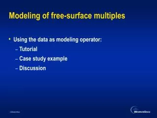
Modeling of free-surface multiples - 2 • Introduction • Long offset Faroes data: velocity analysis and demultiple • Modeling of free-surface multiple diffractions, 3D geometry • Further work
12 km Pre-stack time migration Top basalt Intra basalt Base basalt West East
Line 105 - 1999 data Top basalt Intra basalt Base basalt 7.5 km
Line 104 - 1998 data 7.5 km
Improved results from 1999 data • Better multiple attenuation and velocity analysis • Facilitated by small shot spacing, single cable • Pre-stack time migration • Tested on small area • Clayton’s migration-velocity analysis • Depth migration (coherency analysis and Kirchhoff) • Demultiple using Delft’s SRME
Clayton’s Migration-Velocity Analysis • Slant stack • Downward continuation of the wave field • Convergence criterion: • Input Velocity = Output image
Depth-Velocity model Top B Intra-B Base-B
WBM TBM TB WBM WBM SRME in Shot Gather Domain WB TB TBM WBM TBM Input Input-Predicted multiples Predicted multiples
D() = P () + D ()( r W()-1 )P () Pi(,s,g) = D (,s,g) - ( r W()-1 ) Sx D(, s,x)P i-1(,x,g) x1 x2
Further work (from last week’s seminar) • Effect of position errors (non-coincident sources and receivers) on synthetics: • Use source and receiver positions from the field data; • Specifications for maximum feathering during acquisition • …..
Modeling, diffracted multiples, 3-D • Reference: Taylor & Johnston, Edinburgh Univ, SEG-99 • ``Fast 2-D synthetic seismograms for testing multiple removal’’
Modeling, diffracted multiples, 3-D • With free-surface multiples:
Test cases for the modeling program: • 1 diffractor, no free-surface • 1 diffractor, free-surface • 2 diffractors, no free-surface • 2 diffractors, free-surface
Further work • Investigate effect of feathering on demultiple for the long offset Faroes data • Corrections during computation of the multiple model • Tolerance on feathering • Look at interpolation of missing near offset traces using Radon transforms and SEP’s optimization libraries