Download
1 / 19
190 likes | 310 Views
Levels of Processor/Memory Hierarchy. Can be Modeled by Increasing Dimensionality of Data Array. Additional dimension for each level of the hierarchy. Envision data as reshaped to reflect increased dimensionality.

E N D
Levels of Processor/Memory Hierarchy • Can be Modeled by Increasing Dimensionality of Data Array. • Additional dimension for each level of the hierarchy. • Envision data as reshaped to reflect increased dimensionality. • Calculus automatically transforms algorithm to reflect reshaped data array. • Data, layout, data movement, and scalarization automatically generated based on reshaped data array.
Levels of Processor/Memory Hierarchycontinued • Math and indexing operations in same expression • Framework for design space search • Rigorous and provably correct • Extensible to complex architectures Mathematics of Arrays y= conv (x) Map Approach Example: “raising” array dimensionality < 0 1 2 > x: < 0 1 2 … 35 > < 3 4 5 > P0 Main Memory < 6 7 8 > < 9 10 11 > L2 Cache < 12 13 14 > L1 Cache < 15 16 17 > P1 Memory Hierarchy Map: < 18 19 20 > < 21 22 23 > < 24 25 26 > < 27 28 29 > P2 Parallelism < 30 31 32 > < 33 34 35 >
Application DomainSignal Processing Pulse Compression Doppler Filtering Beamforming Detection 3-d Radar Data Processing Composition of Monolithic Array Operations Convolution Matrix Multiply Change algorithmto better match hardware/memory/communication. Lift dimension algebraically • Hardware Info: • - Memory • - Processor Algorithm is Input Architectural Information is Input Model processors(dim=dim+1); Model time-variance(dim=dim+1); Model Level 1 cache(dim=dim+1) Model All Three: dim=dim+3
Convolution: PSI Calculus Description < 0 0 1 2 . . . > < 0 1 2 3 . . . > < 1 2 3 4 . . . > < 0 0 1 > < 0 1 2 > < 1 2 3 > < 0 0 7 > < 0 6 14 > < 5 12 21 > Definition of y=conv(h,x) y[n]= where x‘has N elements, h has M elements, 0≤n<N+M-1, andx’ is x padded by M-1 zeros on either end Psi Calculus Algorithm step Algorithm and PSI Calculus Description x= < 1 2 3 4 > h= < 5 6 7 > Initial step x= < 1 2 3 4 > h= < 5 6 7 > Form x’ x’= x’=cat(reshape(<k-1>, <0>), cat(x, reshape(<k-1>,<0>)))= < 0 0 1 . . . 4 0 0 > rotate x’ (N+M-1) times x’ rot= x’ rot=binaryOmega(rotate,0,iota(N+M-1), 1 x’) take the size of h part of x’rot x’ final= x’ final=binaryOmega(take,0,reshape<N+M-1>,<M>,=1,x’ rot Prod= multiply Prod=binaryOmega (*,1, h,1,x’ final) sum Y=unaryOmega (sum, 1, Prod) < 7 20 38 . . . > Y= PSI Calculus operators compose to form higher level operations
Experimental Platform and Method Hardware • DY4 CHAMP-AV Board • Contains 4 MPC7400’s and 1 MPC 8420 • MPC7400 (G4) • 450 MHz • 32 KB L1 data cache • 2 MB L2 cache • 64 MB memory/processor Software • VxWorks 5.2 • Real-time OS • GCC 2.95.4 (non-official release) • GCC 2.95.3 with patches for VxWorks • Optimization flags: -O3 -funroll-loops -fstrict-aliasing Method • Run many iterations, report average, minimum, maximum time • From 10,000,000 iterations for small data sizes, to 1000 for large data sizes • All approaches run on same data • Only average times shown here • Only one G4 processor used • Use of the VxWorks OS resulted in very low variability in timing • High degree of confidence in results
Convolution and Dimension Lifting • Model Processor and Level 1 cache. • Start with 1-d inputs(input dimension). • Envision 2nd dimension ranging over output values. • Envision Processors • Reshaped into a 3rd dimension. • The 2nd dimension is partitioned. • Envision Cache • Reshaped into a 4th dimension. • The 1st dimension is partitioned. • “psi” Reduce to Normal Form
Envision 2nd dimension ranging over output values. • Let tz=N+M-1 • M=th=4 • N=tx 4 x S h3 h2 h1 h0 0 0 0 x0 tz tz
- Envision Processors • Reshaped into a 3rd dimension. • The 2nd dimension is partitioned. Let p = 2 -4 -4 - -4- x x S S tz tz 2 2 2
Envision Cache • Reshaped into a 4th dimension • The 1st dimension is partitioned. x x S S 2 2 S S 2 2 x x 2 2 tz/2 tz 2 Tz/2 Tz/2 2
ONF for the Convolution Decomposition with Processors & Cache Generic form- 4 dimensional after “psi” Reduction • For i0= 0 to p-1 do: • For i11= 0 to tz/p –1 do: • sum 0 • For icacherow= 0 to M/cache -1 do: • For i3 = 0 to cache –1 do: • sum sum + h [(M-((icacherow* cache) + i3))-1]* x’[(((tz/p * i0)+i1) + icacherow* cache) + i3)] Let tz=N+M-1 M=th N=tx P r o c e s s o r l o o p C a c h e l o o p T I m e l o o p sum is calculated for each element of y. Time Domain
Outline • Overview • Array Algebra: MoA and Index Calculus: Psi Calculus • Time Domain Convolution • Other algorithms in Radar • Modified Gram-Schmidt QR Decompositions • MOA to ONF • Experiments • Composition of Matrix Multiplication in Beamforming • MoA to DNF • Experiments • FFT • Benefits of Using Moa and Psi Calculus
Algorithms in Radar Mechanize Using Expression Templates Time DomainConvolution (x,y) ONF for 1proc • Lift dimension • - Processor • - L1 cache • reformulate Use toreason about RAW Manual description & derivation for 1 processor DNF DNF ONF Thoughtson an Abstract Machine Modified Gram SchmidtQR (A) ImplementDNF/ONFFortran 90 CompilerOptimizationsDNF to ONF Benchmark at NCSAw/LAPACK A x (BH x C) Beamforming MoA & y Calculus
Benefits of Using Moa and Psi Calculus • Processor/Memory Hierarchy can be modeled by reshaping data using an extra dimension for each level. • Composition of monolithic operations can be reexpressed as composition of operations on smaller data granularities • Matches memory hierarchy levels • Avoids materialization of intermediate arrays. • Algorithm can be automatically(algebraically) transformed to reflect array reshapings above. • Facilitates programming expressed at a high level • Facilitates intentional program design and analysis • Facilitates portability • This approach is applicable to many other problems in radar.
ONF for the QRDecomposition with Processors & Cache Initialization ProcessorLoop ComputeNorm MainLo o p ProcessorLoop Normalize ProcessorCache Loop DoTProduct Processor CacheLoop Ortothogonalize Modified Gram Schmidt
DNF for the Composition of A x (BH x C) Generic form- 4 dimensional • Z=0 • For i=0 to n-1 do: • For j=0 to n-1 do: • For k=0 to n-1 do: • z[k;]z[k;]+A[k;j]xX[j;i]xB[i;] Given A, B, X, Z n by n arrays Beamforming
Typical C++ Operator Overloading Example: A=B+C vector add 2 temporary vectors created Main 1. Pass B and C references to operator + Additional Memory Use B&, C& • Static memory • Dynamic memory (also affects execution time) Operator + 2. Create temporary result vector 3. Calculate results, store in temporary 4. Return copy of temporary temp B+C temp Additional Execution Time temp copy 5. Pass results reference to operator= • Cache misses/page faults • Time to create anew vector • Time to create a copy of a vector • Time to destructboth temporaries temp copy & Operator = temp copy A 6. Perform assignment
C++ Expression Templates and PETE Parse Tree Expression Type Expression + BinaryNode<OpAdd, Reference<Vector>, Reference<Vector > > ExpressionTemplates A=B+C C B Main Parse trees, not vectors, created Parse trees, not vectors, created 1. Pass B and Creferences to operator + Reduced Memory Use B&, C& Operator + • Parse tree only contains references 2. Create expressionparse tree + B& C& 3. Return expressionparse tree copy Reduced Execution Time 4. Pass expression treereference to operator • Better cache use • Loop fusion style optimization • Compile-time expression tree manipulation copy & Operator = 5. Calculate result andperform assignment B+C A • PETE, the Portable Expression Template Engine, is available from theAdvanced Computing Laboratory at Los Alamos National Laboratory • PETE provides: • Expression template capability • Facilities to help navigate and evaluating parse trees PETE: http://www.acl.lanl.gov/pete
Implementing Psi Calculus with Expression Templates take 4 drop rev 3 B size=4 A[i]=B[-i+6] size=7 A[i] =B[-(i+3)+9] =B[-i+6] size=10 A[i] =B[-i+B.size-1] =B[-i+9] size=10 A[i]=B[i] Example: A=take(4,drop(3,rev(B))) B=<1 2 3 4 5 6 7 8 9 10> A=<7 6 5 4> Recall: Psi Reduction for 1-d arrays always yields one or more expressions of the form: x[i]=y[stride*i+ offset] l ≤ i < u 1. Form expression tree 3. Apply Psi Reduction rules 2. Add size information take size=4 drop 4 size=7 Reduction Size info rev 3 size=10 size=10 B 4. Rewrite as sub-expressions with iterators at the leaves, and loop bounds information at the root • Iterators used for efficiency, rather than recalculating indices for each i • One “for” loop to evaluate each sub-expression iterator: offset=6stride=-1 size=4