Download
1 / 24
240 likes | 328 Views
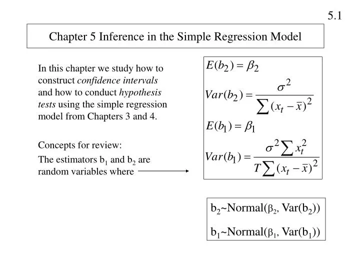
Chapter 5 Inference in the Simple Regression Model. In this chapter we study how to construct confidence intervals and how to conduct hypothesis tests using the simple regression model from Chapters 3 and 4. Concepts for review: The estimators b 1 and b 2 are random variables where.

E N D
Chapter 5 Inference in the Simple Regression Model In this chapter we study how to construct confidence intervals and how to conduct hypothesis tests using the simple regression model from Chapters 3 and 4. Concepts for review: The estimators b1 and b2 are random variables where b2~Normal(2, Var(b2)) b1~Normal(1, Var(b1))
Interval Estimation Least Squares gives us point estimates for 1 and 2. Need to address the issue of precision using knowledge of • the variance of b2 and • the shape of b2’s probability distribution We can construct a margin for error around the point estimates. Review Confidence Intervals: We know that 95% of all possible values for a normal random variable lie within 1.96 standard deviations of the mean 0.025 0.025 0.95 b2 2
where Note that the above interval makes a probabilistic statement about the width of the interval, not about 2 If we knew , then we would have no problem constructing the interval: However, is unknown and must be estimated. This adds an additional source of uncertainty to the interval and also changes the shape of the standardized distribution.
The Student t-distribution We know how to estimate : However, when we standardize b2 using an estimate of , we no longer have a standard normal random variable. Instead we have a random variable with a t-distribution: But: what is se(b2) ??
About the Student t-distribution Compare a z random variable to a t random variable: 1) In the expression for z, the only random variable is b2 z has the same distribution as b2 because 2 and b2 are constants. The distribution is Normal. 2) In the expression for t, b2 and se(b2) are random variables where b2has a normal distribution and se(b2) is a function of which has a 2 distribution. The ratio of a normal random variable to a 2 random variable has a t-distribution.
More on the t t-values have a measure of degrees of freedom. For a simple regression model, this is T – 2. See Table 2 front cover of book. Suppose T = 40 38 d.o.f and 95% of the values lie within 2.024 of the mean. Identify the relevant area on the diagram.
Confidence Intervals Using the t-Distribution 2.024 is the critical t value that leaves 2.5% of the values in the tails. It’s value depends on the degrees of freedom and the level of confidence. A confidence interval for b2 has the general form:
Example of a Confidence Interval In Chapter 3 we found for the food expenditure example: In Chapter 4 we found for the food expenditure example:
This is the 95% confidence interval. There is A 95% probability that this interval contains the true value of 2.
Hypothesis Testing The Idea: • A hypothesis is a conjecture about a population parameter such as “we believe the marginal propensity to spend on food is $0.10 out of every dollar” 2 = 0.10 • Remember that population parameters are unknown constants. • We “test” hypotheses about 2 using b2, our estimator of 2. • b2 is calculated using a sample of data. If b2 is “reasonably” close to the hypothesized value for 2, then we say that the data support the hypothesis. If b2 is NOT “reasonably” close, then we say that the data do not support the hypothesis.
Formal Hypothesis Testing y = 1 + 2x + e 1) Null Hypothesis: specify a value for the parameter Ho: 2 = c where c can be any value. For example, let c = 0, then the Null Hypothesis becomes Ho: 2 = 0. Note that if this were true, then it says that x has no effect on y. This test is called a test of significance.
Alternative Hypothesis: a logical alternative to the Null Hypothesis because if we reject the Null Hypothesis, then we must be prepared to accept the Alternative Hypothesis. Typically, it is H1: 2 c or H1: 2 < c or H1: 2 > c. If we have a test of significance where Ho: 2 = 0, then the Alternative Hypothesis is: H1: 2 0 or H1: 2 < 0 or H1: 2 > 0 Whether we use , < or > depends on the situation and economic theory. For example, it is theoretically impossible that 2 < 0 where 2 is the marginal propensity to consume. Therefore, a test of significance would be: Ho: 2 = 0 H1: 2 > 0
Test Statistic: we use a statistic to “test” the hypothesis. The idea: if the test statistic “disagrees” with the Ho reject Ho. Whether or not the test statistic agrees or disagrees with Ho must be addressed in probabilistic terms. Our test statistic is based on b2. The mean of b2 is 2 but 2 is unknown. *** Make this assumption: Ho is true. Suppose Ho: 2 = c we now know that b2’s distribution is centered at c. This is our test statistic. What do we do with it ?????
4) The Rejection Region: We have assumed the Ho to be true examine the distribution of b2 under this hypothesis. Suppose that we calculate our test statistic and it falls into the tail of this distribution. There are 2 reasons why this might happen: • The assumption that Ho is true is a bad one (meaning the true distribution is centered at a value other than c) • The Hoistrue but our sample data were very unlikely (came from the tail) Extreme values are those values that fall into the tails, depending on the alternative hypothesis. We typically use the 5% most extreme values; a region of low probability. 2 = c b2 0 t
Suppose Ho: 2 = 0 H1: 2 0 The test statistic is The rejection region will be t values that fall into either tail: Two Tailed Test because H1: 2 0. If we use a 5% level of significance, then we put 2.5% into each tail. What t-values leave 0.025 in the tail? Use t-table. Suppose T=40 so that we have 38 degrees of freedom. 0.025 0.025 2=0 b2 0 t
Suppose Ho: 2 = 0 H1: 2 > 0 The test statistic is The rejection region will be t values that fall into the right tail: One Tailed Test If we use a 5% level of significance, then we put 5% into the right tail What t-values leave 0.05 in the tail? Use t-table. Suppose T=40 so that we have 38 degrees of freedom. 0.05 2=0 b2 0 t
5) Conduct the Test: Compare the t-statistic to the rejection region and conclude whether the data fail to reject or reject the null hypothesis (Ho) Example: Food Expenditure Ho: 2 = 0 H1: 2 > 0 Conclusion??
6) Think about Possible Errors We never know for sure whether we have made an error because the truth is never revealed to us. We can only analyze the probability of making an error. When we set our level of significance, we are actually setting the probability of a Type I error. Why? Suppose that Ho is true 5% of the time we will get samples of data that generate a test statistic t that lies in the rejection region, leading us to reject Ho when in fact it is true. We can make the probability of a Type I error smaller by using a 1% level of significance instead of 5%
A Type II Error occurs when we fail to reject Ho when in fact it is false (meaning the alternative hypothesis H1 is true.). In order to measure the probability of this error occurring we need a more specific H1
P-Values As an alternative to specifying the level of significance for a test, we can calculate the p-value of the test, which stands for “probability” value. It is simply the probability of getting the sample test statistic or something more extreme under the assumption that Ho is true. Suppose Ho: 2 = 0 H1: 2 > 0 and our b2 = 0.1283 • P-value is P(b2 0.1283) = P(t 4.20) = area in right tail. In Excel, use this formula: =TDIST(4.2,38,1) 2=0 0.1283 b2 0 4.20 t
For a two-tailed test, we multiply the p-value by 2 Suppose Ho: 2 = 0 H1: 2 0 and our b2 = 0.1283 • P-value is 2 x P(b2 0.1283) = 2 x P(t 4.20) = In Excel, use this formula =TDIST(4.2,38,2)
Least Squares Predictor • This “predictor” is a random variable because it is a function of b1 and b2 which are random variables. • Suppose x = xo, the model predicts • The error is • The variance of this error tells us about the precision of the prediction:
An estimator of var(f) uses an estimator for 2 We can now construct a confidence interval for our predictor Example:
The Idea Behind of Hypothesis Testing • The probability distribution for b2 is centered at β2, which is an unknown parameter. [Remember that E(b2) = β2]. • Assume a value for β2. The value we assume is the value of β2 in the null hypothesis. By assuming a value, we tie down the distribution for b2 (we center the distribution for b2 at the assumed value for β2.) • Use a sample of data on X and Y to calculate the b2 estimate. • Take this value of b2 and match it up to the distribution from 2) above. Does the value of b2 fall near the center of the distribution or out into the tails? If it falls near the center, then this value of b2 has a high probability of occurring under the assumed β2 value; therefore, the assumed value is said to be consistent with the data. If on the other hand, the b2 value falls into the tails, then we say that it has a low probability of occurring under the assumed value; therefore, the assumed value is not consistent with the data. Now, we just need to clarify what it means to be out into the tails or near the center…….this is determined by setting a significance level and the rejection region.