Download

1 / 29
400 likes | 597 Views
Divide-and-Conquer Algorithms. Briana B. Morrison With thanks to Dr. Hung. Divide and Conquer. The most well known algorithm design strategy: Divide instance of problem into two or more smaller instances Solve smaller instances recursively

E N D
Divide-and-ConquerAlgorithms Briana B. Morrison With thanks to Dr. Hung
Divide and Conquer The most well known algorithm design strategy: • Divide instance of problem into two or more smaller instances • Solve smaller instances recursively • Obtain solution to original (larger) instance by combining these solutions
Divide-and-conquer technique a problem of size n subproblem 1 of size n/2 subproblem 2 of size n/2 a solution to subproblem 1 a solution to subproblem 2 a solution to the original problem
Divide and Conquer Examples • Searching: binary search • Sorting: mergesort • Sorting: quicksort • Tree traversals • Matrix multiplication-Strassen’s algorithm
General Divide and Conquer recurrence: Master Theorem T(n) = aT(n/b) + f (n)where f (n)∈Θ(nk) • a < bk T(n) ∈Θ(nk) • a = bk T(n) ∈Θ(nk lg n ) • a > bk T(n) ∈Θ(nlog b a) Note: the same results hold with O and Ω.
Binary Search • Binary search is an efficient algorithm for searching in a sorted array. • Search requires the following steps: 1. Inspect the middle item of an array of size N. 2. Inspect the middle of an array of size N/2. 3. Inspect the middle item of an array of size N/power(2,2) and so on until N/power(2,k) = 1. • This implies k = log2N • k is the number of partitions.
Binary Search • Requires that the array be sorted. • Rather than start at either end, binary searches split the array in half and works only with the half that may contain the value. • This action of dividing continues until the desired value is found or the remaining values are either smaller or larger than the search value.
Binary Search • BinarySearch (List, target, N) • //list: the elements to be searched • //target: the value being searched for • //N: the number of elements in the list • Start = 1 • End = N • While start <= end do • Middle = (start + end) /2 • Select (compare (list [middle], target)) from • Case -1: strat = middle + 1 • Case 0: return middle • Case 1: end = middle – 1 • End select • End while • Return 0
Binary Search • Suppose that the data set is n = 2k - 1sorted items. • Each time examine middle item. If larger, look left, if smaller look right. • Second ‘chunk’ to consider is n/2 in size, third is n/4, fourth is n/8, etc. • Worst case, examine k chunks. n = 2k – 1 so, k = log2(n + 1). (Decision binary tree: one comparison on each level) • Best case, O(1). (Found at n/2). • Thus the algorithm is O(log(n)). • Extension to non-power of 2 data sets is easy.
Binary Search • Best case : O(1) • Worst case : O(log2N) (why?) • Average Case : O(log2N)/2 = O(log2N) (why?)
Mergesort • Mergesort is a recursive sort algorithm. Algorithm: • Split array A[1...n] in two and make copies of each half in arrays B[1... n/2 ] and C[1... n/2 ] • Sort arrays B and C
Mergesort • Merge sorted arrays B and C into array A as follows: • Repeat the following until no elements remain in one of the arrays: • compare the first elements in the remaining unprocessed portions of the arrays • copy the smaller of the two into A, while incrementing the index indicating the unprocessed portion of that array • Once all elements in one of the arrays are processed, copy the remaining unprocessed elements from the other array into A.
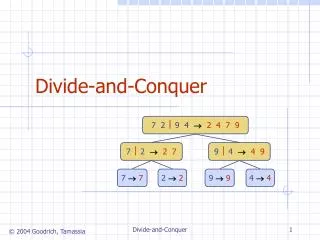
Mergesort Example 7 2 1 6 4 5 3 9
Mergesort … • Algorithm Mergesort (A[0 … n – 1]) • //sorts array A[0 … n – 1] by recursive mergesort • //Input: an array A[0 … n – 1] of orderable elements • //Output: array A[0 … n – 1] sorted in nondecreasing order • If n > 1 • copy A[0 …n/2] to B[0 …n/2 – 1] • copy A[n/2 … n - 1] to C[0 …n/2 – 1] • Mergesort (B[0 …n/2 – 1]) • Mergesort (C[0 …n/2 – 1]) • Merge(B, C, A)
Efficiency of mergesort • C(n) = 2C(n/2) + Cmerge(n) for n > 1, C(1) = 0 • The worst case: • W(n) = 2W(n/2) + n – 1 for n > 1, W(1) = 0
Efficiency of mergesort • All cases have same efficiency: Θ( n log n) • Number of comparisons is close to theoretical minimum for comparison-based sorting: • log n ! ≈ n lg n - 1.44 n • Space requirement: Θ( n ) • Can be implemented without recursion (bottom-up)
Efficiency of Mergesort • Merge analysis (McConnell): • Case 1: where all of the elements of list A are smaller than the first element of list B. • Case 2: what if the first element of A is greater than the first element of B but all of the elements of A are smaller than the second element of B? • Case 3: consider what happens if the elements of A and B are “interleaved” based on their value. In other words, what happens if the value of A[1] is between B[1] and B[2], the value of A[2] is between B[2] and B[3], the value of A[3] is between B[3] and B[4], and so on. • Which is the best case? Worst case?
p A[i]≤p A[i]>p Quicksort • Select a pivot (partitioning/pivot element) • Rearrange the list so that all the elements in the positions before the pivot are smaller than or equal to the pivot and those after the pivot are larger than the pivot (See algorithm Partition/PivotList in section 4.2) • Exchange the pivot with the last element in the first (i.e., ≤ sublist) – the pivot is now in its final position • Sort the two sublists
Quicksort algorithm • Algorithm Quicksort (A[l … r]) • If l < r • s ← partition (A[l … r]) // s is a split position • Quicksort (A[l … s – 1]) • Quicksort (A[s + 1 … r])
Quicksort … • An efficient method based on two scans of the subarray used in the algorithm. • Three situations may arise: • 1) if scanning indices i and j have not crossed, i.e., i < j, we simply exchange A[i] and A[j] and resume the scans. • 2) if the scanning indices have crossed over, i.e., i > j, we have partitioned the array after exchanging the pivot with A[j]. (n + 1 comparisons) • 3) if the scanning indices stop while pointing to the same element, i.e., i = j, the value they are pointing to must be equal to p. Thus, the array is partitioned. (n comparisons)
Quicksort Example 15 22 13 27 12 10 20 25
Efficiency of Quicksort • PivotList analysis: • Case 1: when PivotList creates two parts that are the same size. • Case 2: when the lists are of drastically different sizes. For example, the largest difference in the size of these two lists occurs if the PivotValue is smaller (or larger) than all of the other values in the list. In that case, we wind up with one part that has no elements and the other that has N – 1 elements. What is the number of comparisons? • W(N) = ? • Which is the best case? Worst case?
Efficiency of quicksort • Best case: split in the middle — Θ( n log n) (why?) • Worst case: sorted array! — Θ( n2) (why?) • Average case: random arrays —Θ( n log n) (why?) • Improvements: • better pivot selection: median of three partitioning avoids worst case in sorted files • switch to insertion sort on small subfiles • elimination of recursion these combine to 20-25% improvement • Considered the method of choice for internal sorting for large files (n ≥ 10000)
Strassen’s matrix multiplication • Strassen observed [1969] that the product of two matrices can be computed as follows: C00 C01 A00 A01 B00 B01 = * C10 C11 A10 A11 B10 B11 M1 + M4 - M5 + M7 M3 + M5 = M2 + M4 M1 + M3 - M2 + M6
Submatrices: • M1 = (A00 + A11) * (B00 + B11) • M2 = (A10 + A11) * B00 • M3 = A00 * (B01 - B11) • M4 = A11 * (B10 - B00) • M5 = (A00 + A01) * B11 • M6 = (A10 - A00) * (B00 + B01) • M7 = (A01 - A11) * (B10 + B11)
Efficiency of Strassen’s algorithm • If n is not a power of 2, matrices can be padded with zeros • Number of multiplications: • Number of additions: • Other algorithms have improved this result, but are even more complex
Determining Thresholds • Because recursion requires a fair amount of overhead, • Want to find a value for n where it is at least as fast to call an alternative algorithm as it is to divide the instance further. • Values depend on • Divide and conquer algorithm • Alternative algorithm • Computer which they are implemented
When Not to Use Divide-and-Conquer • Avoid divide-and-conquer in the following situations: • An instance of size n is divided into two or more instances each almost of size n. • An instance of size n is divided into almost n instances of size n/c, where c is a constant.