Download
1 / 25
270 likes | 297 Views
Divide and Conquer Algorithms. Sathish Vadhiyar. Introduction. One of the important parallel algorithm models The idea is to decompose the problem into parts solve the problem on smaller parts find the global result using individual results

E N D
Divide and Conquer Algorithms Sathish Vadhiyar
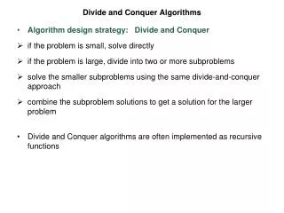
Introduction • One of the important parallel algorithm models • The idea is to • decompose the problem into parts • solve the problem on smaller parts • find the global result using individual results • Works naturally and works well for parallelization
Introduction • Various models • Recursive sub-division: Has a division and computation phase, then a merge phase. E.g., merge sort • Local compute – merge/coordinate – local compute. E.g., following algorithms
Recursive sub-division: • Merge sort (you know already) • Solving tri-diagonal systems
Parallel solution of linear system with special matricesTridiagonal Matrices x1 x2 x3 . . xn b1 b2 b3 . . bn a1 h1 g2 a2 h2 g3 a3 h3 gn an = In general: gixi-1 + aixi + hixi+1 = bi Substituting for xi-1 and xi+1 in terms of {xi-2, xi} and {xi, xi+2} respectively: Gixi-2 + Aixi + Hixi+2 = Bi
Tridiagonal Matrices x1 x2 x3 . . xn B1 B2 B3 . . Bn A1 H1 A2 H2 G3 A3 H3 G4 A4 H4 Gn-2 An = Reordering:
Tridiagonal Matrices x2 x4 . xn x1 x3 . xn-1 B2 B4 . Bn B1 B3 . Bn-1 A2 H2 G4 A4 H4 Gn An A1 H1 G3 A3 H3 Gn-3 An-1 =
Tridiagonal Systems • Thus the problem of size n has been split into even and odd equations of size n/2 • This is odd–even reduction • For parallelization, each process can divide the problem into subproblems of smaller size and solve the subproblems • This is divide-and-conquer technique
Tridiagonal Systems - Parallelization • At each stage one representative process of the domain of processes is chosen • This representative performs the odd-even reduction of problem i to two problems of size i/2 • The problems are distributed to 2 representatives n 1 n/2 2 6 n/4 1 3 5 7 n/8 1 2 3 4 5 6 7 8
Local compute – merge – local compute • Prefix Computations • Sample sort
Parallel Algorithm: Prefix computations on arrays • Array X partitioned into subarrays • Local prefix sums of each subarray calculated in parallel • Prefix sums of last elements of each subarray written to a separate array Y • Prefix sums of elements in Y are calculated. • Each prefix sum of Y is added to corresponding block of X • Divide and conquer strategy
Example 123456789 • 456 789 1,3,6 4,9,15 7,15,24 6,15,24 6,21,45 1,3,6,10,15,21,28,36,45 Divide Local prefix sum Passing last elements to a processor Computing prefix sum of last elements on the processor Adding global prefix sum to local prefix sums in each processor
Lessons Learned.. • Has local computations • Global communication/coordination • Back to local computations
Parallel Sorting by Regular Sampling (PSRS) • Each processor sorts its local data • Each processor selects a sample vector of size p-1; kth element is (n/p * (k+1)/p) • Samples are sent and merge-sorted on processor 0 • Processor 0 defines a vector of p-1 splitters starting from p/2 element; i.e., kth element is p(k+1/2); broadcasts to the other processors
PSRS • Each processor sends local data to correct destination processors based on splitters; all-to-all exchange • Each processor merges the data chunk it receives
Step 5 • Each processor finds where each of the p-1 pivots divides its list, using a binary search • i.e., finds the index of the largest element number larger than the jth pivot • At this point, each processor has p sorted sublists with the property that each element in sublist i is greater than each element in sublist i-1 in any processor
Step 6 • Each processor i performs a p-way merge-sort to merge the ith sublists of p processors
Analysis • The first phase of local sorting takes O((n/p)log(n/p)) • 2nd phase: • Sorting p(p-1) elements in processor 0 – O(p2logp2) • Each processor performs p-1 binary searches of n/p elements – plog(n/p) • 3rd phase: Each processor merges (p-1) sublists • Size of data merged by any processor is no more than 2n/p (proof) • Complexity of this merge sort 2(n/p)logp • Summing up: O((n/p)logn)
Analysis • 1st phase – no communication • 2nd phase – p(p-1) data collected; p-1 data broadcast • 3rd phase: Each processor sends (p-1) sublists to other p-1 processors; processors work on the sublists independently
Analysis Not scalable for large number of processors Merging of p(p-1) elements done on one processor; 16384 processors require 16 GB memory
Sorting by Random Sampling • An interesting alternative; random sample is flexible in size and collected randomly from each processor’s local data • Advantage • A random sampling can be retrieved before local sorting; overlap between sorting and splitter calculation
Sources/References • On the versatility of parallel sorting by regular sampling. Li et al. Parallel Computing. 1993. • Parallel Sorting by regular sampling. Shi and Schaeffer. JPDC 1992. • Highly scalable parallel sorting. Solomonic and Kale. IPDPS 2010.