Download

1 / 40
410 likes | 423 Views
Divide & Conquer Algorithms. Part 2. QuickSort. Worst time: ( n 2 ) Expected time: ( n lg n ) Constants in the expected time are small Sorts in place. QuickSort (cont).

E N D
Divide & Conquer Algorithms Part 2
QuickSort • Worst time: (n2) • Expected time: (nlgn) • Constants in the expected time are small • Sorts in place
QuickSort (cont) • DIVIDE – Partition A[p..r] into two subarrays A[p..q-1] and A[q+1..r] such that each element of A[p..q-1] is A[q] each element of A[q+1..r] • Conquer – Sort the two subarrays by recursive calls to Quicksort • Combine – Since subarrays are sorted in place, they are already sorted
QuickSort (cont) To sort entire array: QuickSort( A, 1, length(A) ) QuickSort( A, p, r ) • if p < r • q Partition( A, p, r ) • QuickSort( A, p, q-1 ) • QuickSort( A, q+1, r )
QuickSort (cont) Partition( A, p, r ) x A[ r ] i p – 1 for j p to r-1 if A[ j ] x i i + 1 Exchange( A[ i ], A[ j ] ) Exchange( A[ i+1 ], A[ r ] ) return i+1
QuickSort (cont) Return i+1 which is 4
Performance of QuickSort • Partition function’s running time - (n) • Running time of QuickSort depends on the balance of the partitions • If balanced, QuickSort is asymptotically as fast as MergeSort • If unbalanced, it is asymptotically as bad as Insertion Sort
Performance of QuickSort (cont) • Worst-case Partitioning • Partitions always of size n-1 and 0 • Occurs when array is already sorted • Recurrence for the running time:
cn cn c(n-1) c(n-1) n c(n-2) c(n-2) c . . . Performance of QuickSort (cont) Total: (n2)
Performance of QuickSort (cont) • Best-case Partitioning • Partitions always of size n/2 and n/2-1 • The recurrence for the running time: Case 2 of Master Method
Performance of QuickSort (cont) • Balanced Partitioning • Average-case is closer to best-case • Any split of constant proportionality (say 99 to 1) will have a running time of (nlgn) • The recurrence will be • Because it yields a recursion tree of depth (lgn), where cost at each level is (n) • See page 151 (new book) for picture • Or next slide
Performance of QuickSort (cont) cn cn log100n c(n/100) c(99n/100) cn c(9801n/10000) c(n/10000) c(99n/10000) c(99n/10000) cn T(1) cn T(1) T(1) T(1) log100/99n cn Total: (nlgn)
Performance of QuickSort (cont) • Intuition for the average case • The behavior depends on the relative ordering of the values • Not the values themselves • We will assume (for now) that all permutations are equally likely • Some splits will be balanced, and some will be unbalanced
Performance of QuickSort (cont) • In a recursion tree for an average-case, the “good” and “bad” splits are distributed randomly throughout the tree • For our example, suppose • Bad splits and good splits alternate • Good splits are best-case splits • Bad splits are worst-case splits • Boundary case (subarray size 0) has cost of 1
n n (n) (n) 0 n - 1 (n-1)/2 (n-1)/2 (n-1)/2-1 (n-1)/2 Performance of QuickSort (cont) • The (n-1) cost of the bad split can be absorbed into the (n) cost of the good split, and the resulting split is good • Thus the running time is (nlgn), but with a slightly larger constant
Randomized QuickSort (1/30/2019) • How do we increase the chance that all permutations are equally likely? • Random Sampling • Don’t always use last element in subarray • Swap it with a randomly chosen element from the subarray • Pivot now is equally likely to be any of the r – p + 1 elements • We can now expect the split to be reasonably well-balanced on average
Randomized QuickSort (cont) Randomized-Partition( A, p, r ) • i Random( p, r ) • Exchange( A[ r ], A[ i ] ) • return Partition( A, p, r ) Note that Partition( ) is same as before
Randomized QuickSort (cont) Randomized-QuickSort( A, p, r ) • if p < r • q Randomized-Partition( A, p, r ) • Randomized-QuickSort( A, p, q-1 ) • Randomized-QuickSort( A, q+1, r )
Analysis of QuickSort • A more rigorous analysis • Begin with worst-case • We intuited that worst-case running time is (n2) • Use substitution method to show this is true
Analysis of QuickSort (cont) • Guess: (n2) • Show: for some c > 0 • Substitute: q2+(n-q-1)2 is max at endpoints of range. Therefore it is • (n-1)2 = n2 – 2n +1
Analysis of QuickSort (cont) • Problem 7.4-1 has you show that • Thus the worst-case running time of QuickSort is (n2)
Analysis of QuickSort (cont) • We will show that the upper-bound on expected running time is (nlgn) • We’ve already shown that the best-case running time is (nlgn) • Combined, these will give an expected running time of (nlgn)
Analysis of QuickSort (cont) • Expected Running Time • Work done is dominated by Partition • Each time a pivot is selected, this element is never included in subsequent calls to QuickSort • And the pivot is in its correct place in the array • Therefore, at most n calls to Partition will be made • Each call to Partition involves (1) work plus the amount of work done in the for loop • Count the total number of times line 4 is executed, we can bound the amount of time spent in the for loop Line 4: if A[j] x
Analysis of QuickSort (cont) • Lemma 7.1 • Let X be the number of comparisons performed in line 4 of Partition over the entire execution of QuickSort on an n-element array. Then the running time of QuickSort is (n + X) • Proof: • There are n calls to Partition, each of which does (1) work then executes the for loop (which includes line 4) some number of times • Since the for loop executes line 4 during each iteration, X represents the number of iterations of the for loop along with the number of comparisons performed • Therefore T(n) = (n (1) + X) = (n + X)
Analysis of QuickSort (cont) • We need to compute X • We do this by computing an overall bound on the total number of comparisons • NOT by computing the number of comparisons at each call to Partition • Definitions: • z1, z2, …, zn elements in the array • zi ith smallest element • set Zij = {zi, zi+1, …, zj}
Analysis of QuickSort (cont) • When does the algorithm compare zi and zj? • Note: each pair of elements is compared at most once. Why? • Our analysis uses indicator random variables
Indicator Random Variables • They provide a convenient method for converting between probabilities and expectations • These are random variables which take on only the value 0 or 1, so they “indicate” whether or not something has happened • Indicator Random Variable I{A} is defined as: • Given a sample space S and an event A • I{A} = 1 if A occurs 0 if A does not occur
Indicator Random Variables (cont) • A simple example • Determine the number of heads when flipping a coin • Sample space S = {H, T} • Simple random variable Y • These are random variables whose range contains only a finite number of elements • In this case, it takes on the values H and T • Each with a probability of ½ • XH is associated with the event Y = H • XH = I{Y = H} = 1 if Y = H 0 if Y = T
Indicator Random Variables (cont) • The expected number of heads in one flip is the expected value of our indicator variable XH • Thus the expected number of heads in one flip is ½
Indicator Random Variables (cont) • Lemma 5.1 • Given a sample space S and an event A in the sample space S, let XA = I{A}. Then E[XA] = Pr{A} • See proof on page 95 • To compute the number of heads in n coin flips • Method 1 – compute the probability of getting 0 heads, 1 heads, 2 heads, etc
Indicator Random Variables (cont) • Method 2 • Let Xi be the indicator random variable associated with the event “the ith flip is heads” • Let Yi be the random variable denoting the outcome of the ith flip • Xi= I{Yi = H} • Let X be the random variable denoting the total number of heads in the n coin flips
Indicator Random Variables (cont) • Take the expectation of both sides: By Lemma 5.1
(Back to) Analysis of QuickSort • We will use indicator random variables • Xij = I{zi is compared to zj} • it indicates whether the comparison took place at any time during execution of QuickSort • Since each pair is compared at most once:
Analysis of QuickSort (cont) • Take expectation of both sides
Analysis of QuickSort (cont) • We still need to compute Pr{ziis compared to zj} • Start by thinking about when two items are not compared • once a pivot x is chosen with zi < x < zj • zi and zj will never be compared • if zi is the first pivot chosen in Zij • zi will be compared to every other element in Zij • Similarly for zj • Thus, zi and zj are compared iff the first pivot from Zij is either zi or zj
Analysis of QuickSort (cont) • What is the probability that this event occurs? • Before a pivot has been chosen from Zij, all elements of Zij are in the same partition • Each element of Zij is equally likely to be chosen as the first pivot • the probability is
Analysis of QuickSort (cont) • Thus we have Because the two events are mutually exclusive
Bound on Harmonic Series: Analysis of QuickSort (cont) Change of variables: k = j – i Note the changes in the summation variables • Combining the two boxed equations
Analysis of QuickSort (cont) • Thus, using Randomized-Partition, the expected running time of QuickSort is (nlgn)