Download
1 / 7
80 likes | 493 Views
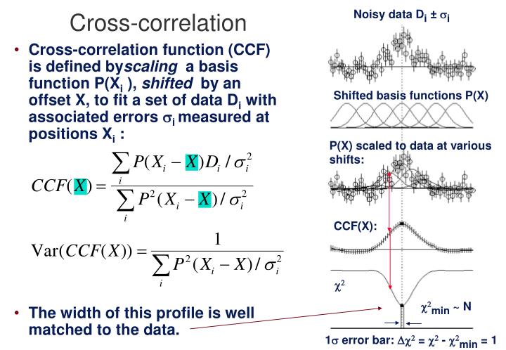
Noisy data D i ± i. Cross-correlation. Cross-correlation function (CCF) is defined by scaling a basis function P(X i ), shifted by an offset X, to fit a set of data D i with associated errors i measured at positions X i : The width of this profile is well matched to the data.

E N D
Noisy data Di ± i Cross-correlation • Cross-correlation function (CCF) is defined byscaling a basis function P(Xi ), shifted by an offset X, to fit a set of data Di with associated errors i measured at positions Xi : • The width of this profile is well matched to the data. Shifted basis functions P(X) P(X) scaled to data at various shifts: CCF(X): min ~ N 1 error bar: = - min = 1
Noisy data Di ± i Mismatched profiles–1 • If basis function has form: • then when width of profile is well matched to the data, correlation length ~ FWHM of minimum ~ . • If profile is too narrow: • CCF has • larger error bars • shorter correlation length • The minimum in is shallow. Profile too narrow P(X) scaled to data at various shifts: CCF(X): min > N Note local minimum causedby nonlinear model Wider 1 error bar: = - min = 1
Noisy data Di ± i Mismatched profiles–2 • If basis function has form: • then when width of profile is well matched to the data, correlation length ~ FWHM of minimum ~ . • If profile is too wide: • CCF has • smaller error bars • longer correlation length • lower peak value • The minimum in is wider, but not as deep. Profile too wide P(X) scaled to data at various shifts: CCF(X): min > N Wider 1 error bar: = - min = 1
Radial velocities from cross-correlation • Data: spectrum of black-hole binary candidateGRO J0422+32 • Basis function: “template” spectrum of normal K5V star of known radial velocity. • Cut out H alpha emission line, fit 5 splines to continuum with ±2 clipping to reject lines.
Wavelength and velocity shifts • Target spectrum Di is measured at wavelengths i and has associated errors i . • Template spectrum P is measured on same (or very similar) wavelength grid. Errors assumed negligible. • For small velocity shift v: Interpolate D i P Note that since D is redshifted relative to P in this example, CCF (v) will produce a peak at positive v. i
Practical considerations • P(X) and D(X) are usually on slightly different wavelength scales so we can’t just shift the spectra bin-by-bin. • We want to measure the CCF as a function of relative velocity, not wavelength. • Velocity shift per bin varies with wavelength: • For each velocity shift in CCF: • Loop over selected range of pixels in target spectrum D(X). • Use pixel wavelength and CCF velocity shift to compute corresponding wavelength in template spectrum P(X) • Use linear interpolation to get flux and variance in template spectrum at this wavelength. • Increment summations and proceed to next pixel in target spectrum.
Radial velocityof GRO J0422+32 • Subtract continuum fit. • Cross-correlate on 6000 A to 6480A subset of data. • Compute CCF for shifts in range ± 1800 km s–1. • CCF shows peak between 500 and 600 km s–1. • Use =1 to get 1 error bar on radial velocity.