Download
1 / 47
650 likes | 909 Views
Correlation. (and a bit on regression). Correlation (Linear). Scatterplots Linear Correlation / Covariance Pearson Product-Moment Correlation Coefficient Factors that Affect Correlation Testing the Significance of a Correlation Coefficient. Correlation.

E N D
Correlation (and a bit on regression)
Correlation (Linear) • Scatterplots • Linear Correlation / Covariance • Pearson Product-Moment Correlation Coefficient • Factors that Affect Correlation • Testing the Significance of a Correlation Coefficient
Correlation • The relationship or association between 2 variables • Is one variable (Y) related to another variable (X)? • Y: criterion variable (DV) • X: predictor variable (IV) • Prediction • ‘Potential’ Causation
Scatterplot (Scatterdiagram, Scattergram) • Pictorial examination of the relationship between two quantitative variables • Each subject is located in the scatterplot by means of a pair of scores (score on the X variable and score on the Y variable) • Predictor variable on the X-axis (abscissa); Criterion variable on the Y-axis (ordinate)
Example of a Scatterplot • The relationship between scores on a test of quantitative skills taken by students on the first day of a stats course (X-axis) and their combined scores on two midterm exams (Y-axis)
Example of a Scatterplot • Here the two variables are positively related - as quantitative skill increases, so does performance on the two midterm exams • Linear relationship between the variables - line of best fit drawn on the graph - the ‘regression line’ • The ‘strength’ or ‘degree’ of the linear relationship is measured by a correlation coefficient i.e. how tightly the data points cluster around the regression line • We can use this information to determine whether the linear relationship represents a true relationship in the population or is due entirely to chance factors
What do we look for in a Scatterplot? • Overall pattern (ellipse!), and any striking deviations (possible outliers**) • Form - is it linear? (curved? clustered?) • Direction - is it positive (high values of the two variables tend to occur together) - or negative (high values of one variable tend to occur with low values of the other variable)? • Strength - how close the points lie to the line of best fit (if a linear relationship)
More Scatterplot Examples An example of the Relationship Between the Scores on the First Midterm (X) and the Scores on the Second Midterm (Y)
More Scatterplot Examples An example of the Relationship Between Order in which a Midterm Is Completed (X) and the Score on the Examination (Y)
Linear Correlation / Covariance • How do we obtain a quantitative measure of the linear association between X and Y? • Pearson Product-Moment Correlation Coefficient, r • Based on a statistic called the covariance - reflects the degree to which the two variables vary together
Covariance • Covariance relates the deviation of each subject’s score on the X variable from the mean of the X scores to the corresponding deviation for that subject on the Y variable • Covariance:
Covariance • Note the similarity between formulas for variance and covariance. Variance measures the deviation of a score (X or Y) from its mean. Covariance measures the degree to which these two sets of deviations vary together,or covary • If the deviations of the X variable and Y variable tend to be of the same size, covariance will be large • If the relationship is inconsistent covariance will be small • e.g. large deviations of X being associated with deviations of various magnitudes on Y, • Where there is no systematic relationship between the two sets of deviations, covariance will be zero
Covariance • Covariance is positive when the signs of the paired deviations on X and Y tend to be the same, and negative when the signs tend to be different. • The sign of covariance determines the direction of association: • positive covariance, r will be positive • negative covariance, r will be negative
The Pearson Product-Moment Correlation Coefficient • r • the ratio of the joint variation of X and Y (covariance) relative to the variation of X and Y considered separately • Conceptually • Values of r near 0 indicate a very weak linear relationship…Values of r close to -1 or +1 indicate that the points lie close to a straight line. The extreme values of -1 and +1 occur only when the points lie exactly along a straight line.
The Pearson Product-Moment Correlation Coefficient • The relationship between IQ scores and grade point average? (N=12 uni students)
Another example • The following slide provides some practice in which you can use the conceptual formula to calculate the correlation coefficient for two subscales of a psychological inventory • See if you can replicate some of the values in the table • You can calculate the means • sx = 4.54 sy= 4.46 • r = .36
Factors Affecting Correlation • Linearity • Range restrictions • Outliers • Beware of spurious correlations….take care in interpretation • High positive correlation between a country’s infant mortality rate and the no. of physicians per 100,000 population
Testing the Significance of a Correlation • In order to make an inference from a correlation coefficient based on a sample of data to the situation in the population…we test a hypothesis using a statistical test • Most commonly, the hypotheses are: • H0: the population correlation (rho ) is zero, = 0 • H1: the population correlation is not zero, ≠ 0
Testing the Significance of a Correlation • The null hypothesis can be tested in several ways, including using a form of t-test. For “significant” correlations use the table in book. Note that df is dealing with pairs so if you have 20 x values and y values your df is n-2 = 18 • E.g. 20 people is tested at time 1 and time 2 • Stat programs produce the probability associated with the computed value of r ie the probability of obtaining that value of r or a more extreme value when H0 is true • We reject H0 when the probability is less than 0.05, however practical considerations come into play once again.
Practical significance • As before with t-tests, larger Ns require smaller critical values for the determination of significance, and perhaps even more so here, statistical significance has limited utility • As we mentioned with effect size, it is best to use the literature of the field of study to determine how strong an effect you are witnessing • e.g. + .50 maybe very strong in some cases • In fact, r provides us with a measure of effect size when conducting regression analysis…
Other correlation calculations • The Spearman Correlation • Ordinal scale data. (i.e., rank order) • Nonlinear, but consistent relationships • The Point-Biserial Correlation • One variable is interval or ratio, the other is dichotomous. • E.g., Correlation between IQ and gender. • Phi-coefficient • Both variables are dichotomous
Advantages of Correlational studies • Show the amount (strength) of relationship present • Can be used to make predictions about the variables studied • Often easier to collect correlational data, and interpretation is fairly straightforward.
Linear Correlation and Linear Regression - Closely Linked • Linear correlation refers to the presence of a linear relationship between two variables ie a relationship that can be expressed as a straight line • Linear regression refers to the set of procedures by which we actually establish that particular straight line, which can then be used to predict a subject’s score on one of the variables from knowledge of the subject’s score on the other variable
The Properties of a Straight Line • Two important numerical quantities are used to describe a straight line: • the slope and the intercept
The Slope • Slope (gradient) - the angle of a line’s tilt relative to one of the axes • Slope = • Slope is the amount of difference in Y associated with 1 unit of difference in X
Slope • A positive slope indicates that the Y variable changes in the same direction as X(eg as X increases, Y increases) • A negative slope indicates that the Y variable changes in the direction opposite to X (eg as X increases, Y decreases)
Intercept • The point at which the line crosses the Y axis at X = 0 (Y intercept) • The Y intercept can be either positive or negative, depending on whether the line intersects the Y axis above the 0 point (positive) or below it (negative)
The Formula for a Straight Line • Only one possible straight line can be drawn once the slope and Y intercept are specified • The formula for a straight line is: • Y = bx + a • Y = the calculated value for the variable on the vertical axis • a = the intercept • b = the slope of the line • X = a value for the variable on the horizontal axis • Once this line is specified, we can calculate the corresponding value of Y for any value of X entered
The Line of Best Fit • Real data do not conform perfectly to a straight line • The best fit straight line is that which minimizes the amount of variation in data points from the line (least squares regression line) • The equation for this line can be used to predict or estimate an individual’s score on Y solely on the basis of his or her score on X
Conceptually • So in the Y=bX+a formula…
To draw the regression line, choose two convenient values of X (often near the extremes of the X values to ensure greater accuracy)and substitute them in the formula to obtain the corresponding Y values, and then plot these points and join with a straight line • With the regression equation, we now have a means by which to predict a score on one variable given the information (score) of another variable • E.g. SAT score and collegiate GPA
Example Serotonin Levels and Aggression in Rhesus Monkeys
The Scatter plot follows. It is clear that an imperfect, linear, negative relationship exists between the two variables.
r-squared - the coefficient of determination • The square of the correlation, r², is the percentage of the variability in the values of y that is explained by the regression of y on x • r² = variance of predicted values y variance of observed values y • When you report a regression, give r² as a measure of how successful the regression was in explaining the result…and when you see a correlation, square it to get a better feel for the strength of the association • Stated differently r2 is a measure of effect size
r2 A Venn Diagram Showing r2 as the Proportion of Variability Shared by Two Variables (X and Y) • The shaded portion shared by the two circles represents the proportion of shared variance: the larger the area of overlap, the greater the strength of the association between the two variables