Download
1 / 53
540 likes | 608 Views
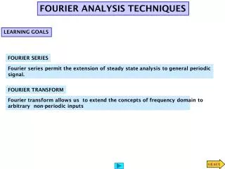
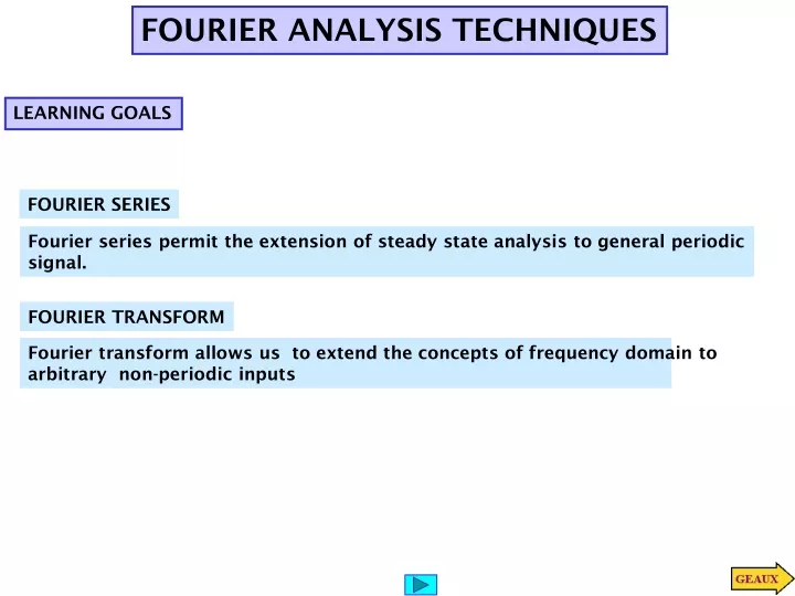
FOURIER ANALYSIS TECHNIQUES. LEARNING GOALS. FOURIER SERIES. Fourier series permit the extension of steady state analysis to general periodic signal. FOURIER TRANSFORM. Fourier transform allows us to extend the concepts of frequency domain to arbitrary non-periodic inputs. FOURIER SERIES.

E N D
FOURIER ANALYSIS TECHNIQUES LEARNING GOALS FOURIER SERIES Fourier series permit the extension of steady state analysis to general periodic signal. FOURIER TRANSFORM Fourier transform allows us to extend the concepts of frequency domain to arbitrary non-periodic inputs
FOURIER SERIES The Fourier series permits the representation of an arbitrary periodic signal as a sum of sinusoids or complex exponentials Periodic signal The smallest T that satisfies the previous condition is called the (fundamental) period of the signal
Phasor for n-th harmonic FOURIER SERIES RESULTS Cosine expansion Complex exponential expansion Trigonometric series Relationship between exponential and trigonometric expansions GENERAL STRATEGY: . Approximate a periodic signal using a Fourier series . Analyze the network for each harmonic using phasors or complex exponentials . Use the superposition principle to determine the response to the periodic signal
Approximation with 4 terms Approximation with 2 terms Approximation with 100 terms Original Periodic Signal EXAMPLE OF QUALITY OF APPROXIMATION
EXPONENTIAL FOURIER SERIES Any “physically realizable” periodic signal, with period To, can be represented over the interval by the expression The sum of exponential functions is always a continuous function. Hence, the right hand side is a continuous function. Technically, one requires the signal, f(t), to be at least piecewise continuous. In that case, the equality does not hold at the points where the signal is discontinuous Computation of the exponential Fourier series coefficients
LEARNING EXAMPLE Determine the exponential Fourier series
LEARNING EXTENSION Determine the exponential Fourier series
LEARNING EXTENSION Determine the exponential Fourier series
Even function symmetry Odd function symmetry TRIGONOMETRIC FOURIER SERIES Relationship between exponential and trigonometric expansions The trigonometric form permits the use of symmetry properties of the function to simplify the computation of coefficients
TRIGONOMETRIC SERIES FOR FUNCTIONS WITH EVEN SYMMETRY TRIGONOMETRIC SERIES FOR FUNCTIONS WITH ODD SYMMETRY
FUNCTIONS WITH HALF-WAVE SYMMETRY Examples of signals with half-wave symmetry Each half cycle is an inverted copy of the adjacent half cycle There is further simplification if the function is also odd or even symmetric
LEARNING EXAMPLE Find the trigonometric Fourier series coefficients This is an even function with half-wave symmetry
LEARNING EXAMPLE Find the trigonometric Fourier series coefficients This is an odd function with half-wave symmetry Use change of variable to show that the two integrals have the same value
LEARNING EXAMPLE Find the trigonometric Fourier series coefficients
LEARNING EXTENSION Determine the type of symmetry of the signals
Determine the trigonometric Fourier series expansion LEARNING EXTENSION
Half-wave symmetry Determine the trigonometric Fourier series expansion LEARNING EXTENSION
1. PSPICE schematic LEARNING EXAMPLE VPWL_FILE in PSPICE library piecewise linear periodic voltage source Determine the Fourier Series of this waveform File specifying waveform Fourier Series Via PSPICE Simulation 1. Create a suitable PSPICE schematic 2. Create the waveform of interest 3. Set up simulation parameters 4. View the results
Use transient analysis comments Fundamental frequency (Hz) Text file defining corners of piecewise linear waveform
Schematic used for Fourier series example To view result: From PROBE menu View/Output File and search until you find the Fourier analysis data Accuracy of simulation is affected by setup parameters. Decreases with number of cycles increases with number of points
FOURIER COMPONENTS OF TRANSIENT RESPONSE V(V_Vs) DC COMPONENT = -1.353267E-08 HARMONIC FREQUENCY FOURIER NORMALIZED PHASE NORMALIZED NO (HZ) COMPONENT COMPONENT (DEG) PHASE (DEG) 1 1.000E+00 4.222E+00 1.000E+00 2.969E-07 0.000E+00 2 2.000E+00 1.283E+00 3.039E-01 1.800E+02 1.800E+02 3 3.000E+00 4.378E-01 1.037E-01 -1.800E+02 -1.800E+02 4 4.000E+00 3.838E-01 9.090E-02 4.620E-07 -7.254E-07 5 5.000E+00 1.079E-04 2.556E-05 1.712E-03 1.711E-03 6 6.000E+00 1.703E-01 4.034E-02 1.800E+02 1.800E+02 7 7.000E+00 8.012E-02 1.898E-02 -9.548E-06 -1.163E-05 8 8.000E+00 8.016E-02 1.899E-02 5.191E-06 2.816E-06 9 9.000E+00 5.144E-02 1.218E-02 -1.800E+02 -1.800E+02 10 1.000E+01 1.397E-04 3.310E-05 1.800E+02 1.800E+02 11 1.100E+01 3.440E-02 8.149E-03 -1.112E-04 -1.145E-04 12 1.200E+01 3.531E-02 8.364E-03 1.800E+02 1.800E+02 13 1.300E+01 2.343E-02 5.549E-03 1.800E+02 1.800E+02 14 1.400E+01 3.068E-02 7.267E-03 -3.545E-05 -3.960E-05 15 1.500E+01 3.379E-04 8.003E-05 -3.208E-03 -3.212E-03 16 1.600E+01 2.355E-02 5.579E-03 -1.800E+02 -1.800E+02 17 1.700E+01 1.309E-02 3.101E-03 2.905E-04 2.854E-04 18 1.800E+01 1.596E-02 3.781E-03 -5.322E-05 -5.856E-05 19 1.900E+01 1.085E-02 2.569E-03 -1.800E+02 -1.800E+02 20 2.000E+01 2.994E-04 7.092E-05 1.800E+02 1.800E+02 TOTAL HARMONIC DISTORTION = 3.378352E+01 PERCENT * file pwl1.txt * example 14.5 * BECA 7 * ORCAD 9.1 * By J.L. Aravena 0,0 0.1,1 0.2,3 0.3,6 0.4,3 0.5,0 0.6,-3 0.7,-6 0.8,-3 0.9,-1 1.0,0 RELEVANT SEGMENT OF OUTPUT FILE
LEARNING EXAMPLE It is easier to study the effect of time-shift with the exponential series expansion TIME-SHIFTING Time shifting the function only changes the phase of the coefficients
Time shifting and half-wave periodic signals Only the odd coefficients of f1 are used
It was shown before that for v(t) LEARNING EXTENSION
WAVEFORM GENERATION Time scaling does not change the values of the series expansion Time-shifting modifies the phase of the coefficients If the Fourier series for f(t) is known then one can easily determine the expansion for any time-shifted and time-scaled version of f(t) The coefficients of a linear combination of signals are the linear combination of the coefficients One can tabulate the expansions for some basic waveforms and use them to determine the expansions or other signals
Signals with Fourier series tabulated in BECA 7
From the table of Fourier series Use the table of Fourier series to determine the expansions of these functions LEARNING EXTENSION Strictly speaking the value for n=0 must be computed separately.
The amplitude spectrum displays Dn as the function of the frequency. The phase spectrum displays the angle as function of the frequency. The frequency axis is usually drawn in units of fundamental frequency The two-sided spectrum is based on the exponential representation In the two-sided case, the amplitude spectrum plots |cn| while the phase spectrum plots versus frequency (in units of fundamental frequency) Both spectra display equivalent information FREQUENCY SPECTRUM The spectrum is a graphical display of the coefficients of the Fourier series. The one-sided spectrum is based on the representation
Phase spectrum Amplitude spectrum LEARNING EXAMPLE The Fourier series expansion, when A=5, is given by Determine and plot the first four terms of the spectrum
From the table of series LEARNING EXTENSION Determine the trigonometric Fourier series and plot the first four terms of the amplitude and phase spectra
STEADY STATE NETWOK RESPONSE TO PERIODIC INPUTS 1. Replace the periodic signal by its Fourier series 2. Determine the steady state response to each harmonic 3. Add the steady state harmonic responses
AVERAGE POWER In a network with periodic sources (of the same period) the steady state voltage across any element and the current through are all of the form The average power is the sum of the average powers for each harmonic
Determine the average power LEARNING EXTENSION
FOURIER TRANSFORM A heuristic view of the Fourier transform A non-periodic function can be viewed as the limit of a periodic function when the period approaches infinity
Determine the Fourier transform LEARNING EXAMPLE For comparison we show the spectrum of a related periodic function
LEARNING EXTENSION Determine LEARNING EXAMPLES Determine the Fourier transform of the unit impulse function
Change integration variable Proof of the convolution property Exchanging orders of integration And limits of integration remain the same
LEARNING EXTENSION From the table of transforms (And all initial conditions are zero) A Systems application of the convolution property The output (response) of a network can be computed using the Fourier transform Use partial fraction expansion!
Think of f(t) as a voltage applied to a one Ohm resistor By definition, the left hand side is the energy of the signal Intuitively, if the Fourier transform has a large magnitude over a frequency range then the signal has significant energy over that range And if the magnitude of the Fourier transform is zero (or very small) then the signal has no significant energy in that range PARSEVAL’S THEOREM Parseval’s theorem permits the determination of the energy of a signal in a given frequency range
Examine the effect of this low-pass filter in the quality of the input signal LEARNING BY APPLICATION One can use Bode plots to visualize the effect of the filter High frequencies in the input signal are attenuated in the output The effect is clearly visible in the time domain
The output signal is slower and with less energy than the input signal
Effect of band-pass filter Effect of low-pass filter Effect of band-stop filter Effect of high-pass filter EFFECT OF IDEAL FILTERS
Ideal filter to tune out one AM station Proposed tuning circuit Fourier transform of received signal LEARNING BY DESIGN “Tuning-out” an AM radio station Fourier transform of signal broadcast by two AM stations Next we show how to design the tuning circuit by selecting suitable R,L,C
Design equations Frequency response of circuit tuned to 960kHz Ideal filter to tune out one AM station Design specifications Fourier transform of received signal Designing the tuning circuit More unknowns than equations. Make some choices
LEARNING EXAMPLE noise noise Proposed two-stage band-pass with two identical stages An example of band-pass filter signal Design requirement: Make the signal 100 times stronger than the noise