Download
1 / 32
650 likes | 1.4k Views
Fourier analysis. Fourier analysis. Fourier analysis describes the process of breaking a function into a sum of simpler pieces. R ebuilding the function from these pieces is known as synthesis

E N D
Fourier analysis • Fourier analysis describes the process of breaking a function into a sum of simpler pieces. • Rebuilding the function from these pieces is known as synthesis • Fourier analysis has been extended over time to apply to more and more abstract and general situations, and the general field is often known as harmonic analysis. • Each transform used for analysis (see list of Fourier-related transforms) has a corresponding inverse transform that can be used for synthesis
Fourier analysis - Applications • Fourier analysis has many scientific applications in: • Physics, • Partial differential equations, • Number theory, • Combinatorics, • Signal processing, • Imaging, • Probability theory, • Statistics, • Option pricing, • Cryptography, • Numerical analysis, • Acoustics, • Oceanography, • Optics, • Diffraction, • Geometry, and other areas.
Fourier analysis - Applications • This wide applicability stems from many useful properties of the transforms: • The transforms are linear operators. • The transforms are usually invertible, and when they are, the inverse transform has a similar form as the forward transform. • in a linear time-invariant physical system, frequency is a conserved quantity, so the behavior at each frequency can be solved independently. • Fourier transforms turn the complicated convolution operation into simple multiplication, which means that they provide an efficient way to compute convolution-based operations such as polynomial multiplication and multiplying large numbers. • The discrete version of the Fourier transform can be evaluated quickly on computers using fast Fourier transform (FFT) algorithms. • Fourier transformation is also useful as a compact representation of a signal.
Applications in signal processing • When processing signals, such as audio, radio waves, light waves, seismic waves, and even images, Fourier analysis can isolate individual components of a compound waveform, concentrating them for easier detection and/or removal. • A large family of signal processing techniques consist of Fourier-transforming a signal, manipulating the Fourier-transformed data in a simple way, and reversing the transformation. • Examples include: • Telephone dialing; the touch-tone signals for each telephone key, when pressed, are each a sum of two separate tones. • Removal of unwanted frequencies from an audio recording • Noise gating of audio recordings to remove quiet background noise by eliminating Fourier components that do not exceed a preset amplitude; • Equalization of audio recordings with a series of band pass filters; • Digital radio reception with no superheterodyne circuit, as in a modern cell phone or radio scanner; • Image processing to remove periodic artifacts • Cross correlation of similar images for co-alignment; • X-ray crystallography to reconstruct a protein's structure from its diffraction pattern; • Fourier transform ion cyclotron resonance mass spectrometry to determine the mass of ions from the frequency of cyclotron motion in a magnetic field.
Variants of Fourier analysis • Fourier analysis has different forms, some of which have different names.
Fourier transform • Fourier series is used for analysing continous aperiodic signals • Fourier transform describes a function ƒ(t) in terms of basic complex exponentials of various frequencies. • Fourier transform is given by the complex number: • Evaluating this quantity for all values of omega produces the frequency-domain function.
Fourier series • Used for the analysis for functions defined on a circle, or equivalently for periodic functions. • Suppose that ƒ(x) is periodic function with period 2π, in this case one can attempt to decompose ƒ(x) as a sum of complex exponentials functions. • The coefficients of the complex exponential in the sum are referred to as the Fourier coefficients for ƒ and are given by: • And the Fourier series of ƒ(x) is given by:
Discrete-time Fourier transform (DTFT) • Used to analyse discrete aperiodic signals • Discrete-time Fourier transform (DTFT) provides a useful frequency-domain transform. • A useful "discrete-time" function can be obtained by sampling a "continuous-time" function, s(t), which produces a sequence, s(nT), for integer values of n and some time-interval T. • The DTFT is obtained from: • Applications of the DTFT are not limited to sampled functions. • It can be applied to any discrete sequence.
Discrete Fourier transform (DFT) • Used to analyse discrete periodic signals • when s[n] is periodic, with period N, formula for the coefficients simplifies to: • The inverse transform of S[k] does not produce the finite-length sequence, s[n], when evaluated for all values of n. • Therefore it is often said that the DFT is a transform for Fourier analysis of finite-domain, discrete-time functions. • The DFT can be computed using a fast Fourier transform (FFT) algorithm, which makes it a practical and important transformation on computers. for all integer values of k.
Interpretation in terms of Time and Frequency • In signal processing, the Fourier transform often takes a time domain signal and maps it into a frequency domain signal. • It is a decomposition of a function into sinusoids of different frequencies; in the case of a Fourier series or discrete Fourier transform, the sinusoids are harmonics of the fundamental frequency of the function being analyzed.
Properties of the Fourier Transform • Time Shifting/Reversal • Scaling Time • Frequency Shifting • Duality • Convolution • Correlation • Modulation • Differentials
Time Shifting/Reversal • Remember • If • The Fourier transform of this is simply: • If time is reversed, all that happens in the Fourier integral in the e -jωt term becomes e -jω (-t) = e jωt, which is merely the complex conjugate of e -jωt. • Therefore, provided f (t) is real, the Fourier integral will be the complex conjugate. Where Time reversal is indicated by a # superscript
Scaling Time • All that is needed is to make the substitution u = k t, and du = k dt, in the Fourier integral:
Frequency Shifting • Scaling frequency is equally simple:
Frequency Shifting Example • Let's multiply an arbitrary function f (t) by an infinite series of Dirac impulse functions and replace the impulse train by its Fourier series to get. • We have merely replaced a sum to infinity over time of delta functions, with a sum to infinity over frequency of exponentials. • Each of these terms is of the form e-jωt f(t), which is a frequency shift giving F(ω - Ω ): • We therefore have F(ω) repeated to infinity at intervals of 2π / Ts, and hence the frequency spectrum is repeated at intervals of 2π / Ts on the frequency axis.
Duality • Lets take the Fourier integral, and compare it to the inverse Fourier integral: • Let's express the second integral slightly differently: • If we replace ta by -ω and ωa by t, then we get the integral • From above we can see that if we can do a transform one way, we can do it the other way easily! Just replace t by -ω and ω by t, and multiply the function in terms of ω by 2π, and you're there.
Convolution • The Fourier transform translates between convolution and multiplication of functions. • Fourier transforms turn the complicated convolution operation into simple multiplication, which means that they provide an efficient way to compute convolution-based operations. • If ƒ(x) and h(x) are integrable functions with Fourier transforms F(ω) and H(ω) and y(x) = ƒ(x) * h(x) Then Y(ω) = F(ω)H(ω) • In linear time invariant (LTI) system theory, it is common to interpret h(x) as the impulse response of an LTI system with input ƒ(x) and output y(x), since substituting the unit impulse for ƒ(x) yields y(x) = h(x). • In this case, represents the frequency response of the system. • Conversely: y(x) = ƒ(x)h(x) Then Y(ω) = F(ω)*H(ω)
Correlation • If y(x) is the cross-correlation of ƒ(x) andh(x) y(x) = ƒ(x) *h(x) then Y(ω) = Ĥ(ω)F(ω) • This property is important in signal processing because it can be used to detect a known signal in the presence of noise as well as for noise removal.
Modulation • For any real number x0, if h(x) = ƒ(x − x0), then H(ω) = e-2πix0ωF(ω) • A delay in time results in the multiplication of the frequency spectrum by another frequency a process called frequency translation. • For any real number ω0, if h(x) = e2πixω0ƒ(x), then H(ω) = F(ω – ω0) • Multiplication of two time domain signals which is modulation, results in a delay in the frequency spectrum.
Differentials • Fourier transforms, and the closely related Laplace transforms are widely used in solving differential equations. • If f(x) is a differentiable function with Fourier transform F(ω), then the Fourier transform of its derivative is given by : 2πiωF(ω) • In a linear time-invariant physical system, frequency is a conserved quantity, so the behavior at each frequency can be solved independently.
The Ideal Low pass Filters Amplitude response/Magnitude frequency response • The ideal low pass filter is characterized by a gain of 1 for all frequencies below some cut-off frequency in normalized Hz, and a gain of 0 for all higher frequencies. • It is sometimes called a high-cut filter, or treble cut filter when used in audio applications. • Low-pass filters play the same role in signal processing that moving averages do in some other fields, such as finance. • An ideal low-pass filter can be realized mathematically (theoretically) by multiplying a signal by the rectangular function in the frequency domain or, equivalently, convolution with a sinc function in the time domain.
The Ideal Low pass Filters • The impulse response of the ideal low pass filter is: • The impulse response is infinitely long in time, noncausal and cannot be shifted to make it causal. • Compromise in the design of any practical lowpass filter. Sinc x = sin πx/πx
Bode Plot • A Bode magnitude plot is a graph of log magnitude versus frequency, plotted with a log-frequency axis, to show the transfer function or frequency response of a linear, time-invariant system. • With the magnitude gain being logarithmic, Bode plots make multiplication of magnitudes a simple matter of adding
Bode Plot • A Bode magnitude plot is a graph of log magnitude versus frequency, plotted with a log-frequency axis, to show the transfer function or frequency response of a linear, time-invariant system.
Filters • Three types of analog filters are commonly used: • Chebyshev • Butterworth • Bessel (also called a Thompson filter). • Each of these is designed to optimize a different performance parameter. • The characteristics of these filters are more important than how they are constructed.
Filter Specifications • Analogue filters are specified in terms of their '3dB point’ and their 'roll off‘ • Digital filters are specified in terms of desired attenuation, and permitted deviations from the desired value in their frequency response. • Digital filters can also have an 'arbitrary response': meaning, the attenuation is specified at certain chosen frequencies, or for certain frequency bands. • Filters are also characterised by their response to an impulse: a signal consisting of a single value followed by zeroes:
Frequency Domain Filtering • Filtering can be done directly in the frequency domain, by operating on the signal's frequency spectrum:
Basic Filter Building Block - Modified Sallen-Key Circuit. Common building block for analog filter design This type of circuit is very common for small quantity manufacturing and R&D applications Cascading 2,3, and 4 of these circuits forms Four, six, and eight pole filters