Download
1 / 36
360 likes | 503 Views
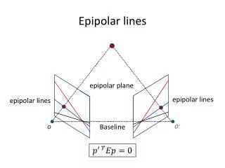
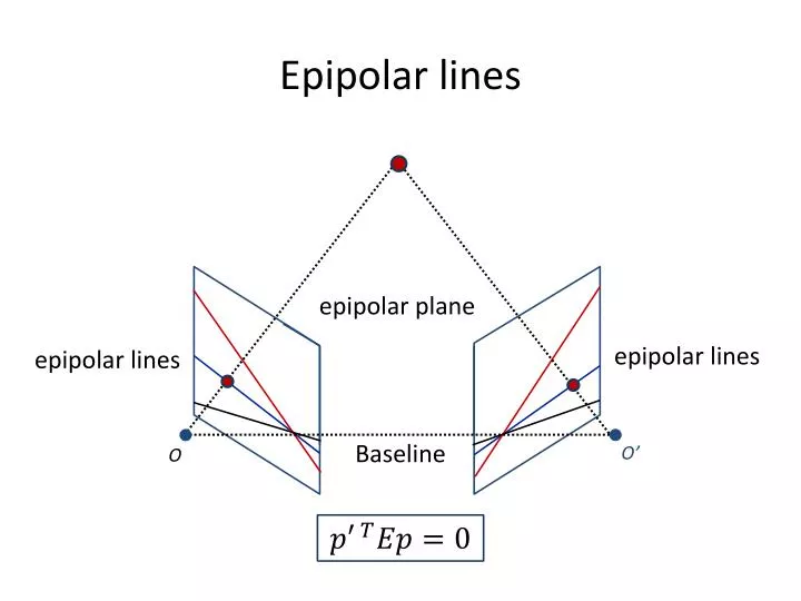
Epipolar lines. epipolar plane. epipolar lines. epipolar lines. Baseline. O’. O. Rectification.

E N D
Epipolar lines epipolar plane epipolar lines epipolar lines Baseline O’ O
Rectification • Rectification: rotation and scaling of each camera’s coordinate frame to make the epipolar lines horizontal and equi-height,by bringing the two image planes to be parallel to the baseline • Rectification is achieved by applying homography to each of the two images
Rectification Baseline O’ O
Cyclopean coordinates • In a rectified stereo rig with baseline of length , we place the origin at the midpoint between the camera centers. • a point is projected to: • Left image: , • Right image: , • Cyclopean coordinates:
Disparity • Disparity is inverse proportional to depth • Constant disparity constant depth • Larger baseline, more stable reconstruction of depth (but more occlusions, correspondence is harder) (Note that disparity is defined in a rectified rig in a cyclopean coordinate frame)
Random dot stereogram • Depth can be perceived from a random dot pair of images (Julesz) • Stereo perception is based solely on local information (low level)
Compared elements • Pixel intensities • Pixel color • Small window (e.g. or ), often using normalized correlation to offset gain • Features and edges (less common) • Mini segments
Dynamic programming • Each pair of epipolar lines is compared independently • Local cost, sum of unary term and binary term • Unary term: cost of a single match • Binary term: cost of change of disparity (occlusion) • Analogous to string matching (‘diff’ in Unix)
String matching • Swing → String S t r i n g Start S w i n g End
String matching • Cost: #substitutions + #insertions + #deletions S t r i n g S w i n g
Dynamic Programming • Shortest path in a grid • Diagonals: constant disparity • Moving along the diagonal – pay unary cost (cost of pixel match) • Move sideways – pay binary cost, i.e. disparity change (occlusion, right or left) • Cost prefers fronto-parallel planes. Penalty is paid for tilted planes
Dynamic Programming Start , Complexity?
Probability interpretation: Viterbi algorithm • Markov chain • States: discrete set of disparity • Log probabilities: product sum
Probability interpretation: Viterbi algorithm • Markov chain • States: discrete set of disparity • Maximum likelihood: minimize sum of negative logs • Viterbi algorithm: equivalent to shortest path
Dynamic Programming: Pros and Cons • Advantages: • Simple, efficient • Achieves global optimum • Generally works well • Disadvantages:
Dynamic Programming: Pros and Cons • Advantages: • Simple, efficient • Achieves global optimum • Generally works well • Disadvantages: • Works separately on each epipolar line, does not enforce smoothness across epipolars • Prefers fronto-parallel planes • Too local? (considers only immediate neighbors)
Markov Random Field • Graph In our case: graph isa 4-connected gridrepresenting one image • States: disparity • Minimize energy of the form • Interpreted as negative log probabilities
Iterated Conditional Modes (ICM) • Initialize states (= disparities) for every pixel • Update repeatedly each pixel by the most likely disparity given the values assigned to its neighbors: • Markov blanket: the state of a pixel only depends on the states of its immediate neighbors • Similar to Gauss-Seidel iterations • Slow convergence to (often bad) local minimum
Graph cuts: expansion moves • Assume is non-negative and is metric: • We can apply more semi-global moves using minimal s-t cuts • Converges faster to a better (local) minimum
α-Expansion • In any one round, expansion move allows each pixel to either • change its state to α, or • maintain its previous state Each round is implemented via max flow/min cut • One iteration: apply expansion moves sequentially with all possible disparity values • Repeat till convergence
α-Expansion • Every round achieves a globally optimal solution over one expansion move • Energy decreases (non-increasing) monotonically between rounds • At convergence energy is optimal with respect to all expansion moves, and within a scale factor from the global optimum: where
α-Expansion (1D example) • But what about?
α-Expansion (1D example) • Such a cut cannot be obtained due to triangle inequality:
Common Metrics • Potts model: • Truncated : • Truncated squared difference is not a metric
Reconstruction with graph-cuts Original Result Ground truth
A different application: detect skyline • Input: one image, oriented with sky above • Objective: find the skyline in the image • Graph: grid • Two states: sky, ground • Unary (data) term: • State = sky, low if blue, otherwise high • State = ground, high if blue, otherwise low • Binary term for vertical connections: • If the state of a node is sky, the node above should also be sky (set to infinity if not) • If the state of a node is ground, the node below should also be ground • Solve with expansion move. This is a binary (two state) problem, and so graph cut can find the global optimum in one expansion move