Download

1 / 56
600 likes | 945 Views
Epipolar geometry Class 5. 3D photography course schedule (tentative). Optical flow. Brightness constancy assumption. (small motion). 1D example. possibility for iterative refinement. Optical flow. Brightness constancy assumption. (small motion). 2D example. the “aperture” problem.

E N D
Optical flow • Brightness constancy assumption (small motion) • 1D example possibility for iterative refinement
Optical flow • Brightness constancy assumption (small motion) • 2D example the “aperture” problem (1 constraint) ? (2 unknowns) isophote I(t+1)=I isophote I(t)=I
Optical flow • How to deal with aperture problem? (3 constraints if color gradients are different) Assume neighbors have same displacement
Lucas-Kanade Assume neighbors have same displacement least-squares:
Revisiting the small motion assumption • Is this motion small enough? • Probably not—it’s much larger than one pixel (2nd order terms dominate) • How might we solve this problem? * From Khurram Hassan-Shafique CAP5415 Computer Vision 2003
Reduce the resolution! * From Khurram Hassan-Shafique CAP5415 Computer Vision 2003
u=1.25 pixels u=2.5 pixels u=5 pixels u=10 pixels image It-1 image It-1 image I image I Gaussian pyramid of image It-1 Gaussian pyramid of image I Coarse-to-fine optical flow estimation slides from Bradsky and Thrun
warp & upsample run iterative L-K . . . image J image It-1 image I image I Gaussian pyramid of image It-1 Gaussian pyramid of image I Coarse-to-fine optical flow estimation slides from Bradsky and Thrun run iterative L-K
Feature tracking • Identify features and track them over video • Small difference between frames • potential large difference overall • Standard approach: KLT (Kanade-Lukas-Tomasi)
Good features to track • Use same window in feature selection as for tracking itself • Compute motion assuming it is small Affine is also possible, but a bit harder (6x6 in stead of 2x2) differentiate:
Example Simple displacement is sufficient between consecutive frames, but not to compare to reference template
Good features to keep tracking Perform affine alignment between first and last frame Stop tracking features with too large errors
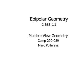
Two-view geometry Three questions: • Correspondence geometry: Given an image point x in the first image, how does this constrain the position of the corresponding point x’ in the second image? • (ii) Camera geometry (motion): Given a set of corresponding image points {xi ↔x’i}, i=1,…,n, what are the cameras P and P’ for the two views? • (iii) Scene geometry (structure): Given corresponding image points xi ↔x’i and cameras P, P’, what is the position of (their pre-image) X in space?
The epipolar geometry C,C’,x,x’ and X are coplanar
The epipolar geometry What if only C,C’,x are known?
The epipolar geometry All points on p project on l and l’
The epipolar geometry Family of planes p and lines l and l’ Intersection in e and e’
The epipolar geometry epipoles e,e’ = intersection of baseline with image plane = projection of projection center in other image = vanishing point of camera motion direction an epipolar plane = plane containing baseline (1-D family) an epipolar line = intersection of epipolar plane with image (always come in corresponding pairs)
Example: motion parallel with image plane (simple for stereo rectification)
The fundamental matrix F algebraic representation of epipolar geometry we will see that mapping is (singular) correlation (i.e. projective mapping from points to lines) represented by the fundamental matrix F
The fundamental matrix F geometric derivation mapping from 2-D to 1-D family (rank 2)
The fundamental matrix F algebraic derivation (note: doesn’t work for C=C’ F=0)
The fundamental matrix F correspondence condition The fundamental matrix satisfies the condition that for any pair of corresponding points x↔x’ in the two images
The fundamental matrix F F is the unique 3x3 rank 2 matrix that satisfies x’TFx=0 for all x↔x’ • Transpose: if F is fundamental matrix for (P,P’), then FT is fundamental matrix for (P’,P) • Epipolar lines: l’=Fx & l=FTx’ • Epipoles: on all epipolar lines, thus e’TFx=0, x e’TF=0, similarly Fe=0 • F has 7 d.o.f. , i.e. 3x3-1(homogeneous)-1(rank2) • F is a correlation, projective mapping from a point x to a line l’=Fx (not a proper correlation, i.e. not invertible)
Fundamental matrix for pure translation General motion Pure translation for pure translation F only has 2 degrees of freedom
The fundamental matrix F relation to homographies valid for all plane homographies
The fundamental matrix F relation to homographies requires
Projective transformation and invariance Derivation based purely on projective concepts F invariant to transformations of projective 3-space unique not unique canonical form
~ ~ Show that if F is same for (P,P’) and (P,P’), there exists a projective transformation H so that P=HP and P’=HP’ ~ ~ Projective ambiguity of cameras given F previous slide: at least projective ambiguity this slide: not more! lemma: (22-15=7, ok)
The projective reconstruction theorem If a set of point correspondences in two views determine thefundamental matrix uniquely, then the scene and cameras may be reconstructed from these correspondences alone, and any two such reconstructions from these correspondences are projectively equivalent allows reconstruction from pair of uncalibrated images!
p p L2 L2 m1 m1 m1 C1 C1 C1 M M L1 L1 l1 l1 e1 e1 lT1 l2 e2 e2 Canonical representation: l2 m2 m2 m2 l2 l2 Fundamental matrix (3x3 rank 2 matrix) C2 C2 C2 Epipolar geometry Underlying structure in set of matches for rigid scenes • Computable from corresponding points • Simplifies matching • Allows to detect wrong matches • Related to calibration
Epipolar geometry? courtesy Frank Dellaert
Other entities besides points? Lines give no constraint for two view geometry (but will for three and more views) Curves and surfaces yield some constraints related to tangency (e.g. Sinha et al. CVPR’04)
Computation of F • Linear (8-point) • Minimal (7-point) • Robust (RANSAC) • Non-linear refinement (MLE, …) • Practical approach
Epipolar geometry: basic equation separate known from unknown (data) (unknowns) (linear)
~10000 ~100 ~10000 ~100 ~10000 ~10000 ~100 ~100 1 Orders of magnitude difference between column of data matrix least-squares yields poor results ! the NOT normalized 8-point algorithm
(0,500) (700,500) (-1,1) (1,1) (0,0) (0,0) (700,0) (-1,-1) (1,-1) the normalized 8-point algorithm Transform image to ~[-1,1]x[-1,1] normalized least squares yields good results(Hartley, PAMI´97)
the singularity constraint SVD from linearly computed F matrix (rank 3) Compute closest rank-2 approximation
the minimum case – 7 point correspondences one parameter family of solutions but F1+lF2 not automatically rank 2