Download
1 / 50
530 likes | 737 Views
Epipolar geometry. Three questions:. Correspondence geometry: Given an image point x in the first view, how does this constrain the position of the corresponding point x’ in the second image?.

E N D
Three questions: • Correspondence geometry: Given an image point x in the first view, how does this constrain the position of the corresponding point x’ in the second image? • Camera geometry (motion): Given a set of corresponding image points {xi ↔x’i}, i=1,…,n, what are the cameras P and P’ for the two views? Or what is the geometric transformation between the views? • (iii) Scene geometry (structure): Given corresponding image points xi ↔x’i and cameras P, P’, what is the position of the point X in space?
The epipolar geometry C,C’,x,x’ and X are coplanar
The epipolar geometry All points on p project on l and l’
The epipolar geometry Family of planes p and lines l and l’ Intersection in e and e’
The epipolar geometry epipoles e,e’ = intersection of baseline with image plane = projection of projection center in other image = vanishing point of camera motion direction an epipolar plane = plane containing baseline (1-D family) an epipolar line = intersection of epipolar plane with image (always come in corresponding pairs)
Calibrated Camera Essential matrix
Uncalibrated Camera Fundamental matrix
Properties of fundamental and essential matrix • Matrix is 3 x 3 • Transpose : If F is essential matrix of cameras (P, P’). FT is essential matrix of camera (P’,P) • Epipolar lines: Think of p and p’ as points in the projective plane then F p is projective line in the right image. That is l’=F p l = FT p’ • Epipole: Since for any p the epipolar line l’=F p contains the epipole e’. Thus (e’T F) p=0 for a all p . Thus e’T F=0 and F e =0
Fundamental matrix • Encodes information of the intrinsic and extrinisic parameters • F is of rank 2, since S has rank 2 (R and M and M’ have full rank) • Has 7 degrees of freedom There are 9 elements, but scaling is not significant and det F = 0
Essential matrix • Encodes information of the extrinisic parameters only • E is of rank 2, since S has rank 2 (and R has full rank) • Its two nonzero singular values are equal • Has only 5 degrees of freedom, 3 for rotation, 2 for translation
Scaling ambiguity Depth Z and Z’ and t can only be recovered up to a scale factor Only the direction of translation can be obtained
Least square approach We have a homogeneous system A f =0 The least square solution is smallest singular value of A, i.e. the last column of V in SVD of A = U D VT
Non-Linear Least Squares Approach Minimize with respect to the coefficients of F Using an appropriate rank 2 parameterization
Locating the epipoles SVD of F = UDVT.
Rectification • Image Reprojection • reproject image planes onto common plane parallel to line between optical centers
Rectification • Rotate the left camera so epipole goes to infinity along the horizontal axis • Apply the same rotation to the right camera • Rotate the right camera by R • Adjust the scale
3D Reconstruction • Stereo: we know the viewing geometry (extrinsic parameters) and the intrinsic parameters: Find correspondences exploiting epipolar geometry, then reconstruct • Structure from motion (with calibrated cameras): Find correspondences, then estimate extrinsic parameters (rotation and direction of translation), then reconstruct. • Uncalibrated cameras: Find correspondences, Compute projection matrices (up to a projective transformation), then reconstruct up to a projective transformation.
Reconstruction by triangulation P’ If cameras are intrinsically and extrinsically calibrated, find P as the midpoint of the common perpendicular to the two rays in space.
Triangulation ap’ ray through C’ and p’, bRp + T ray though C and p expressed in right coordinate system R = ? T = ?
Linear triangulation Linear combination of 2 other equations homogeneous Homogenous system: X is last column of V in the SVD of A= USVT
Geometric error Reconstruct matches in projective frame by minimizing the reprojection error Non-iterative optimal solution
Reconstruction for intrinsically calibrated cameras • Compute the essential matrix E using normalized points. • Select M=[I|0] M’=[R|T] then E=[Tx]R • Find T and R using SVD of E
Decomposition of E E can be computed up to scale factor T can be computed up to sign (EET is quadratic) Four solutions for the decomposition, Correct one corresponds to positive depth values
SVD decomposition of E • E = USVT
Reconstruction from uncalibrated cameras Reconstruction problem: given xi↔x‘i , compute M,M‘ and Xi for all i without additional information possible only up to projective ambiguity
Projective Reconstruction Theorem • Assume we determine matching points xi and xi’. Then we can compute a unique Fundamental matrix F. • The camera matrices M, M’ cannot be recovered uniquely • Thus the reconstruction (Xi) is not unique • There exists a projective transformation H such that
From Projective to Metric Reconstruction • Compute homography H such that XEi=HXi for 5 or more control points XEi with known Euclidean position. • Then the metric reconstruction is
From affine to metric • Use constraints from scene orthogonal lines • Use constraints arising from having the same camera in both images
Reconstruction from N Views • Projective or affine reconstruction from a possible large set of images • Given a set of camera Mi, • For each camera Mi a set of image point xji • Find 3D points Xj and cameras Mi, such that MiXj=xji
Bundle adjustment • Solve following minimization problem • Find Mi and Xj that minimize • Levenberg Marquardt algorithm • Problems many parameters 11 per camera, 3 per 3d point • Useful as final adjustment step for bundles of rays