Download
1 / 17
180 likes | 342 Views
Navy Operational Assimilative Global Ocean Modeling. Dr. Charlie Barron barron@nrlssc.navy.mil Naval Research Laboratory Stennis Space Center. Navy Global Ocean Modeling.

E N D
Navy Operational AssimilativeGlobal Ocean Modeling Dr. Charlie Barron barron@nrlssc.navy.mil Naval Research Laboratory Stennis Space Center
Navy Global Ocean Modeling • The Naval Research Laboratory has developed and transitioned the global ocean modeling system now operational at the Naval Oceanographic Office: • Present system • Key products • Evaluate performance • Future plans
Operational Navy Assimilative Ocean Modeling Global models NCOM, HYCOM Regional models NCOM/NCODA Ocean Prediction acoustics/currents Ocean Analysis NCODA, ISOP
Global NCOM: configuration and references Global NCOM • ~14 km average spacing • 41 vertical σ–z levels stretched logarithmically to 5500 m • 1 m upper layer rest thickness • CICE 3.0 Arctic ice model • NOGAPS wind stress, bulk heat flux • NCODA assimilation of in situ observations Key references: http://www7320.nrlssc.navy.mil/global_ncom/pubs.html Barron et al., JGR Oceans, 2007. drifter evaluation Barron et al., Ocean Modelling, 2006. model formulation Kara et al., Ocean Modelling, 2006. general evaluation Barron et al., J. Atm. Oceanic Techn., 2004. SSH evaluation
Key Products • Key operational products supported by global Navy ocean models include: • Sound speed for acoustic calculations in anti submarine warfare • Boundary conditions for nested ocean models and coupled atmospheric models • Currents for buoy drift, mine drift, search and recovery • Ice products such as ice edge, thickness • Model validation studies focus on these operational products. • New transitions must in some way improve information for key operational products.
Impact of ocean models on sound speed prediction Observed • RMS Range error: 1.7 km • Max Range error: 4.1 km • Present operational synthetic based on SSH, SST: • Fails to represent surface sonic layers • Significant errors in predicting transmission loss Synthetic • RMS Range error: 0.5 km • Max Range error: 1.3 km • Assimilating synthetics into global NCOM: • Dynamics produce a relatively deep mixed layer • Smaller errors in predicting transmission loss GNCOM 0600Hz at 20m depth
Validate model attributes that are relevant to key products Evaluate hydrographic proxies to indicate expected acoustic fidelity: Mixed Layer Depth (MLD) Kara et al. (2000) density threshold equivalent to ΔT=0.8°C Below-Layer Gradient (BLG) Fit a line to sound speed points between SLD and SLD+100m BLG is the slope*100 with units ms-1/100m Negative BLG ↔ downward refraction Positive BLG ↔ upward refraction speed(z) ≈ speed(SLD) + BLG*(z-SLD)/100 Sonic Layer Depth (SLD) Helber et al. (submitted) near surface sound speed maximum appropriate for frequency range
Evaluate NCOM assimilating MLD-modified synthetic vs. synthetic For MLD, where is MLD-modified GNCOM better than a standard synthetic(MODAS)? • 11 m GNCOM median improvement • GNCOM better in 80% of the regions. (shown in red and yellow) Statistics based on 43,474 T,S profiles from 2006.
Evaluate NCOM assimilating MLD-modified synthetic vs. synthetic For MLD, where is MLD-modified GNCOM better than a standard synthetic(MODAS)? • 10 m GNCOM median improvement • GNCOM better in 83% of the regions. (shown in red and yellow) Statistics based on 6,942 unassimilated T,S profiles from 2006.
Validate model attributes that are relevant to key products Median statistics relative to 43,474 T,S profiles over the global ocean. Statistics based on 43,474 T,S profiles from 2006. Profiles are compared with nearest climatology, synthetic, and GNCOM nowcasts. None of the products here assimilate profiles.
Validate model attributes that are relevant to key products Median statistics relative to 6,942 T,S profiles over the Western North Pacific. Statistics based on 6,942 T,S profiles from 2006. Profiles are compared with nearest climatology, synthetic, and GNCOM nowcasts. None of the products here assimilate profiles.
Product example: currents for search and recovery Adam Air flight 574 crashed in the Java Sea on 1 January 2007. USNS Mary Sears assisted in search and recovery, locating black boxes on 21 January. Forward 10-day trajectories starting around crash site NTSB location initial crash debris Pinger Locations Reverse 10-day trajectories starting from debris field EAS NCOM results (nested within global NCOM) guided the search by predicting sources of debris that washed ashore ten days after the crash and evaluating debris distributions from potential crash sites.
RMS separation (km) after one day between observed and simulated drifter trajectories for experiments in 2003. Regions sorted by increasing V. Best results are highlighted in green, second-place in grey. 200,000 + comparisons see Barron et al., J. Geophys Res., 2007.
Assessment Summary • RMS drifter separation after one day • prior operational V2.0 and new V2.5 (1/16° to 1/32° NLOM, no mean correction) • RMS error is linearly proportional to σV. • 8% reduction in prediction uncertainty • 15% reduction in predicted search area
Future Plans Similar metrics are being applied to planned upgrades. Upgrades will transition to operations if they demonstrate improved performance. ISOP New covariances, EOF models to estimate synthetic profiles Global HYCOM • Global HYCOM • ~6.5 km avg. spacing • 32 hybrid layers • Cycling NCODA assimilation • ESMF-coupled CICE
Operational Navy Assimilative Ocean Modeling Summary • Identify key products • Focus on relevant metrics • Establish performance of present system • Demonstrate benefit of potential upgrades