Download
1 / 23
230 likes | 366 Views
The Squared Correlation r 2 – What Does It Tell Us?. Lecture 51 Sec. 13.9 Mon, Dec 12, 2005. Residual Sum of Squares. Recall that the line of “best” fit was that line with the smallest sum of squared residuals. This is also called the residual sum of squares :. Other Sums of Squares.

E N D
The Squared Correlation r2 – What Does It Tell Us? Lecture 51 Sec. 13.9 Mon, Dec 12, 2005
Residual Sum of Squares • Recall that the line of “best” fit was that line with the smallest sum of squared residuals. • This is also called the residual sum of squares:
Other Sums of Squares • There are two other sums of squares associated with y. • The regression sum of squares: • The total sum of squares:
Other Sums of Squares • The regression sum of squares, SSR, measures the variability in y that is predicted by the model, i.e., the variability in y^. • The total sum of squares, SST, measures the observed variability in y.
Example – SST, SSR, and SSE • Plot the data in Example 13.14, p. 800, withy. 20 18 16 14 12 10 8 8 10 12 14 16
Example – SST, SSR, and SSE • The deviations of y fromy (observed). 20 18 16 14 12 10 8 8 10 12 14 16
Example – SST, SSR, and SSE • The deviations of y^ fromy (predicted). 20 18 16 14 12 10 8 8 10 12 14 16
Example – SST, SSR, and SSE • The deviations of y from y^ (residual deviations). 20 18 16 14 12 10 8 8 10 12 14 16
The Squared Correlation • It turns out that • It also turns out that
Explaining Variation • One goal of regression is to “explain” the variation in y. • For example, if x were height and y were weight, how would we explain the variation in weight? • That is, why do some people weigh more than others? • Or if x were the hours spent studying for a math test and y were the score on the test, how would we explain the variation in scores? • That is, why do some people score higher than others?
Explaining Variation • A certain amount of the variation in y can be explained by the variation in x. • Some people weigh more than others because they are taller. • Some people score higher on math tests because they studied more. • But that is never the full explanation. • Not all taller people weigh more. • Not everyone who studies longer scores higher.
Explaining Variation • High degree of correlation between x and y variation in x explains most of the variation in y. • Low degree of correlation between x and y variation in x explains only a little of the variation in y. • In other words, the amount of variation in y that is explained by the variation in x should be related to r.
Explaining Variation • Statisticians consider the predicted variation SSR to be the amount of variation in y (SST) that is explained by the model. • The remaining variation in y, i.e., residual variation SSE, is the amount that is not explained by the model.
Explaining Variation SST = SSE + SSR
Explaining Variation SST = SSE + SSR Total variation in y (to be explained)
Explaining Variation SST = SSE + SSR Total variation in y (to be explained) Variation in y that is explained by the model
Explaining Variation Variation in y that is unexplained by the model SST = SSE + SSR Total variation in y Variation in y that is explained by the model
Example – SST, SSR, and SSE • The total (observed) variation in y. 20 18 16 14 12 10 8 8 10 12 14 16
Example – SST, SSR, and SSE • The variation in y that is explained by the model. 20 18 16 14 12 10 8 8 10 12 14 16
Example – SST, SSR, and SSE • The variation in y that is not explained by the model. 20 18 16 14 12 10 8 8 10 12 14 16
Explaining Variation • Therefore, • r2 is the proportion of variation in y that is explained by the model and 1 – r2 is the proportion that is not explained by the model.
TI-83 – Calculating r2 • To calculate r2 on the TI-83, • Follow the procedure that produces the regression line and r. • In the same window, the TI-83 reports r2.
Let’s Do It! • Let’s Do It! 13.3, p. 819 – Oil-Change Data. • Do part (b) on the TI-83. • How much of the variation in repair costs is explained by frequency of oil change?