Download
1 / 61
710 likes | 1.25k Views
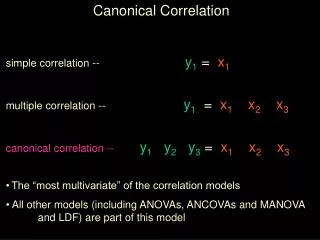
Canonical Correlation. What is Canonical Correlation?. Canonical correlation seeks the weighted linear composite for each variate (sets of D.V.s or I.V.s) to maximize the overlap in their distributions.

E N D
What is Canonical Correlation? • Canonical correlation seeks the weighted linear composite for each variate (sets of D.V.s or I.V.s) to maximize the overlap in their distributions. • Labeling of D.V. and I.V. is arbitrary. The procedure looks for relationships and not causation. • Goal is to maximize the correlation (not the variance extracted as in most other techniques). • Canonical correlation is the “mother” m.v. model • Lacks specificity in interpreting results that may limit its usefulness in many situations
X1 X2 X3 X4 . . . Xq Y1 Y2 Y3 Y4 . . . Yp What is the best way to understand how the variables in these two sets are related?
Bivariate correlations across sets • Multiple correlations across sets • Principal components within sets; correlations between principal components across sets
X1 X2 X3 X4 . . . Xq Y1 Y2 Y3 Y4 . . . Yp What linear combinations of the X variables (u) and the Y variables (t) will maximize their correlation?
b1X1 + b2X2 + b3X3 + b4X4 + . + bpXp =u a1Y1 + a2Y2 + a3Y3 + a4Y4 + . + aqYq = t What linear combinations of the X variables (u) and the Y variables (t) will maximize their correlation?
b1X1 + b2X2 + b3X3 + b4X4 + . + bpXp a1Y1 + a2Y2 + a3Y3 + a4Y4 + . + aqYq Max(Rc) Where Rc represents the overlapping variance between two variates which are linear composites of each set of variables
Assumptions • Multiple continuous variables for D.V.s and I.V.s or categorical with dummy coding • Assumes linear relationship between any two variables and between variates. • Multivariate normality is necessary to perform statistical tests. • Sensitive to homoscedasticity decreases correlation between variables • Multicollinearity in either variate confounds interpretation of canonical results
When use Canonical Correlation? • Descriptive technique which can define structure in both the D.V. and I.V. variates simultaneously • Series of measures are used for both D.V. and I.V. • Canonical correlation also has ability to define structure in each variate, which are derived to maximize their correlation
Objectives of Canonical Correlation • Determine the magnitude of the relationships that may exist between two sets of variables • Derive a variate(s) for each set of criterion and predictor variables such that the variate(s) of each set is maximally correlated. • Explain the nature of whatever relationships exist between the sets of criterion and predictor variables • Seek the max correlation of shared variance between the two sides of the equation
Information: Canonical Functions • Canonical correlation: Correlation between two sets; the largest possible correlation that can be found between linear combinations. • Canonical variate: The linear combinations created from the IV set and DV set. • Extraction of canonical variates can continue up to a maximum defined by the number of measures in the smaller of the two sets.
Information: Canonical Variates • Canonical weights: weights used to create the linear combinations; interpreted like regression coefficients • Canonical loadings: correlations between each variable and its variate; interpreted like loadings in PCA • Canonical cross-loadings: Correlation of each observed independent or dependent variable with opposite canonical variate
Interpreting Canonical Variates • Canonical Weights • Larger weight contributes more to the function • Negative weight indicates an inverse relationship with other variables • Be careful of multicollinearity • Assess stability of samples
Interpreting Canonical Variates • Canonical Loadings – direct assessment of each variable’s contribution to its respective canonical variate • Larger loadings = more important to deriving the canonical variate • Correlation between the original variable and its canonical variate • Assess stability of loadings across samples
Interpreting Canonical Variates • Canonical Cross-Loadings • Measure of correlation of each original D.V. with the independent canonical variate. • Direct assessment of the relationship between each D.V. and the independent variate. • Provides a more pure measure of the dependent and independent variable relationship • Preferred approach to interpretation
Canonical Cross-Loadings Represents the correlation between Y1 and the X variate X1 X2 X3 X4 . . . Xq Y1 Y2 Y3 Y4 . . . Yp
Canonical Loadings and Weights Loading X1: correlation between X1 and X variate (its own variate) X1 X2 X3 X4 . . . Xq Y1 Y2 Y3 Y4 . . . Yp r Weight X1: unique partial contribution of X1 to X variate (its own variate)
Deriving Canonical Functions & Assessing Overall Fit • Max # of variate functions = # of variables in the smallest set - I.V. or D.V. • Variates extracted in steps. Factor which accounts for max residual variance is selected • First pair of canonical variates has the highest intercorrelation possible • Successive pairs of variates are orthogonal and independent of all variates • Canonical correlation squared represents the amount of variance in one canonical variate that is accounted for by the other canonical variate
Interpretation: Selection of Functions • Level of statistical significance of the function – usually F statistic based on Rao’s approximation, p < .05 • Magnitude of the canonical relationship –size of canonical correlations; practical significance • Rc2 variance shared by variates, not variance extracted from predictor & criterion variables • Redundancy index – summary of the ability of a set of predictor variables to account for variation in criterion variables
Redundancy Index Redundancy = [Mean of (loadings)2] x Rc2 • Provides the shared variance that can be explained by the canonical function • Redundancy provided for both IV and DV variates, but DV variate of more interest • Both loadings and Rc2 must be high to get high redundancy
Considerations: Canonical R • Small sample sizes may have an adverse affect • Suggested minimum sample size = 10 * # of variables • Selection of variables to be included: • Conceptual or Theoretical basis • Inclusion of irrelevant or deletion of relevant variables may adversely affect the entire canonical solution • All I.V.s must be interrelated and all D.V.s must be interrelated • Composition of D.V. and I.V. variates is critical to producing practical results
Limitations • Rc reflects only the variance shared by the linear composites, not the variances extracted from the variables • Canonical weights are subject to a great deal of instability • Interpretation difficult because rotation is not possible • Precise statistics have not been developed to interpret canonical analysis
Crosby, Evans, and Cowles (1990) examined the impact of relationship quality on the outcome of insurance sales. They examined relationship characteristics and outcomes for 151 transactions. • Relationship Characteristics: • Appearance similarity • Lifestyle similarity • Status similarity • Interaction intensity • Mutual disclosure • Cooperative intentions
Crosby, Evans, and Cowles (1990) examined the impact of relationship quality on the outcome of insurance sales. They examined relationship characteristics and outcomes for 151 transactions. • Outcomes: • Trust in the salesperson • Satisfaction with the salesperson • Cross-sell • Total insurance sales
Matrix data Variables = rowtype_ trust satis cross total appear life status interact mutual coop . Begin data N 151 151 151 151 151 151 151 151 151 151 Mean 0 0 0 0 0 0 0 0 0 0 STDDEV 1 1 1 1 1 1 1 1 1 1 Corr 1.00 corr .63 1.00 corr .28 .22 1.00 corr .23 .24 .51 1.00 corr .38 .33 .29 .20 1.00 corr .42 .28 .36 .39 .57 1.00 corr .37 .30 .39 .29 .48 .59 1.00 corr .30 .36 .21 .18 .15 .29 .30 1.00 corr .45 .37 .31 .39 .29 .41 .35 .44 1.00 corr .56 .56 .24 .29 .18 .33 .30 .46 .63 1.00 end data.
Variable labels trust ' Trust in the salesperson' Satis 'Satisfaction with the salesperson' cross 'Cross-sell' total 'Total insurance sales' appear 'Appearance similarity' life 'Lifestyle similarity' status 'Status similarity' interact 'Interaction intensity' mutual 'Mutual disclosure' coop 'Cooperative intentions' . MANOVA trust satis cross total with appear life status interact mutual coop /matrix=IN(*) /print signif(multiv dimenr eigen stepdown univ hypoth) error(cor) /discrim raw stan cor alpha(1).
Multivariate Tests of Significance (S = 4, M = 1/2, N = 69 1/2) Test Name Value Approx. F Hypoth. DF Error DF Sig. of F Pillais .73301 5.38481 24.00 576.00 .000 Hotellings 1.35153 7.85574 24.00 558.00 .000 Wilks .37940 6.57954 24.00 493.10 .000 Roys .52771 There is at least one significant relationship between the two sets of measures. With 6 and 4 measures in the two sets, there are a maximum of 4 possible sets of linear combinations that can be formed.
Eigenvalues and Canonical Correlations Root No. Eigenvalue Pct. Cum. Pct. Canon Cor. Sq. Cor 1 1.117 82.672 82.672 .726 .528 2 .176 13.050 95.722 .387 .150 3 .050 3.706 99.428 .218 .048 4 .008 .572 100.000 .088 .008 Rc2 Rc
Dimension Reduction Analysis Roots Wilks L. F Hypoth. DF Error DF Sig. of F 1 TO 4 .37940 6.57954 24.00 493.10 .000 2 TO 4 .80331 2.15996 15.00 392.40 .007 3 TO 4 .94500 1.02566 8.00 286.00 .417 4 TO 4 .99233 .37087 3.00 144.00 .774 Two of the four possible sets of linear combinations are significant.
Standardized canonical coefficients for DEPENDENT variables Function No. Variable 1 2 3 4 TRUST -.543 .317 -.390 1.082 SATIS -.364 -.936 .103 -.816 CROSS -.186 .148 1.160 .057 TOTAL -.239 .721 -.672 -.597 • Outcomes: • Trust in the salesperson • Satisfaction with the salesperson • Cross-sell • Total insurance sales
Correlations between DEPENDENT and canonical variables Function No. Variable 1 2 3 4 TRUST -.879 -.065 -.155 .447 SATIS -.804 -.530 -.048 -.265 CROSS -.540 .399 .731 -.124 TOTAL -.546 .645 -.145 -.515 • Outcomes: • Trust in the salesperson • Satisfaction with the salesperson • Cross-sell • Total insurance sales
Standardized canonical coefficients for COVARIATES CAN. VAR. COVARIATE 1 2 3 4 APPEAR -.268 -.561 .342 .552 LIFE -.164 .833 -.467 .138 STATUS -.156 .128 .906 -.007 INTERACT -.049 -.379 .361 -.853 MUTUAL -.128 .749 -.209 -.441 COOP -.603 -.773 -.566 .408 • Relationship Characteristics: • Appearance similarity • Lifestyle similarity • Status similarity • Interaction intensity • Mutual disclosure • Cooperative intentions
Correlations between COVARIATES and canonical variables CAN. VAR. Covariate 1 2 3 4 APPEAR -.589 -.003 .402 .445 LIFE -.674 .531 .095 .155 STATUS -.622 .267 .660 .052 INTERACT -.517 -.209 .196 -.739 MUTUAL -.729 .319 -.182 -.345 COOP -.855 -.263 -.353 -.120 • Relationship Characteristics: • Appearance similarity • Lifestyle similarity • Status similarity • Interaction intensity • Mutual disclosure • Cooperative intentions
Remaining issues: • How much variance is really accounted for? • How easily does the procedure capitalize on chance?
How much variance is reallyaccounted for? Reliance on the canonical correlations for evidence of variance accounted for across sets of variables can be misleading. Each linear combination only captures a portion of the variance in its own set. That needs to be taken into account when judging the variance accounted for across sets.
The squared canonical correlation indicates the shared variance between linear combinations from the two sets.
Each linear combination accounts for only a portion of the variance in the variables in its set.
Redundancy Index Redundancy = [Mean of (loadings)2] x Rc2 • Provides the shared variance that can be explained by the canonical function • Redundancy provided for both IV and DV variates, but DV variate of more interest • Both loadings and Rc2 must be high to get high redundancy • Proportion of variance in the variables of the opposite set that is accounted for by the linear combination.
Fader and Lodish (1990) collected data for 331 different grocery products. They sought relations between what they called structural variables and promotional variables. The structural variables were characteristics not likely to be changed by short-term promotional activities. The promotional variables represented promotional activities. The major goal was to determine if different promotional activities were associated with different types of grocery products.
Structural variables (X): PENET Percentage of households making at least one category purchase PCYCLE Average interpurchase time PRICE Average dollars spent in the category per purchase occasion PVTSH Combined market share for all private-label and generic products PURHH Average number of purchase occasions per household during the year
Promotional variables (Y): FEAT Percent of volume sold on feature (advertised in local newspaper) DISP Percent of volume sold on display (e.g., end of aisle) PCUT Percent of volume sold at a temporary reduced price SCOUP Percent of volume purchased using a retailer’s store coupon MCOUP Percent of volume purchased using a manufacturer’s coupon
SPSS syntax Canonical correlation analysis must be obtained using syntax statements in SPSS: MANOVA penet purhh pcycle price pvtsh with feat disp pcut scoup mcoup /print signif(multiv dimenr eigen stepdown univ hypoth) error(cor) /discrim raw stan cor alpha(1).
Structural variables (X): PENET Percentage of households making at least one category purchase PCYCLE Average interpurchase time PRICE Average dollars spent in the category per purchase occasion PVTSH Combined market share for all private-label and generic products PURHH Average number of purchase occasions per household during the year Promotional variables (Y): FEAT Percent of volume sold on feature (advertised in local newspaper) DISP Percent of volume sold on display (e.g., end of aisle) PCUT Percent of volume sold at a temporary reduced price SCOUP Percent of volume purchased using a retailer’s store coupon MCOUP Percent of volume purchased using a manufacturer’s coupon PENET PURHH PCYCLE PRICE PVTSH FEAT DISP PCUT SCOUP MCOUP BEER 62.3 11.1 46 5.16 .4 19 32 27 1 1 WINE 42.9 5.8 59 4.58 1.0 14 26 8 0 1 FRESH BREAD 98.6 26.6 21 1.30 39.4 12 4 15 1 2 CUPCAKES 27.4 2.5 60 1.11 3.5 4 10 10 1 4
The same coefficients exist for the other set of variables. Raw canonical coefficients for COVARIATES Function No. COVARIATE 1 2 3 4 5 FEAT .083 -.151 -.058 -.232 .215 DISP .044 .011 .108 .091 .074 PCUT .021 .199 .037 .079 -.247 SCOUP -.015 -.385 -.788 1.124 -.268 MCOUP .022 -.079 .043 -.003 -.057
Test Name Value Approx. F Hypoth. DF Error DF Sig. of F Pillais .73057 11.12256 25.00 1625.00 .000 Hotellings 1.09732 14.01931 25.00 1597.00 .000 Wilks .41262 12.85124 25.00 1193.96 .000 Roys .41271 These tests indicate whether there is any significant relationship between the two sets of variables. They do not indicate how many of those sets of linear combinations are significant. With 5 variables in each set, there are up to 5 sets of linear combinations that could be derived. This test tells us that at least the first one is significant.
Eigenvalues and Canonical Correlations Root No. Eigenvalue Pct. Cum. Pct. Canon Cor. Sq. Cor 1 .703 64.040 64.040 .642 .413 2 .305 27.790 91.830 .483 .234 3 .075 6.877 98.708 .265 .070 4 .013 1.198 99.906 .114 .013 5 .001 .094 100.000 .032 .001 The canonical correlations are extracted in decreasing size. At each step they represent the largest correlation possible between linear combinations in the two sets, provided the linear combinations are independent of any previously derived linear combinations.
Dimension Reduction Analysis Roots Wilks L. F Hypoth. DF Error DF Sig. of F 1 TO 5 .41262 12.85124 25.00 1193.96 .000 2 TO 5 .70257 7.53593 16.00 984.36 .000 3 TO 5 .91682 3.17374 9.00 786.25 .001 4 TO 5 .98600 1.14582 4.00 648.00 .334 5 TO 5 .99897 .33534 1.00 325.00 .563 Procedures for testing the significance of the canonical correlations can be applied sequentially. At each step, the test indicates whether there is any remaining significant relationships between the two sets. In this case, three sets of linear combinations can be formed.
As in principal components, identifying the number of significant sets of linear combinations is just the beginning. The nature of those linear combinations must also be determined. This requires interpreting the canonical weights and loadings.
The linear combinations can be formed using the variables in their original metrics. Sometimes this makes it easier to understand the role a particular variable plays because the metric is well understood. Raw canonical coefficients for DEPENDENT variables Function No. Variable 1 2 3 4 5 PENET .036 -.018 .016 .016 .011 PURHH -.073 -.013 -.175 .072 -.329 PCYCLE -.012 -.031 -.019 .049 -.020 PRICE .198 -.838 -.417 -.299 .305 PVTSH .000 .024 -.061 .002 .039