Download
1 / 40
410 likes | 474 Views
Understand light and surface interaction, create 3-D views, and implement shading in OpenGL. Explore the rendering equation and different light sources for realistic graphics. Learn about specular, diffuse, and translucent surfaces.

E N D
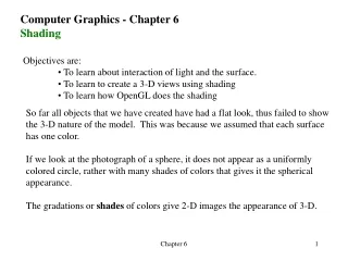
Computer Graphics - Chapter 6 Shading • Objectives are: • To learn about interaction of light and the surface. • To learn to create a 3-D views using shading • To learn how OpenGL does the shading So far all objects that we have created have had a flat look, thus failed to show the 3-D nature of the model. This was because we assumed that each surface has one color. If we look at the photograph of a sphere, it does not appear as a uniformly colored circle, rather with many shades of colors that gives it the spherical appearance. The gradations or shades of colors give 2-D images the appearance of 3-D. Chapter 6
Light and Matter From a physical perspective, a surface can either emit light by self-emission, light bulb and sun, or reflect light from other surfaces that illuminates it. The color that we see on an object may be the result of multiple interactions between light sources and reflective surfaces. Mathematically, the rendering equation is what we need to solve to determine the shading of a surface. There are approximation, ray tracing, and radiosity that may be used to determine the shade. But, none of these methods are efficient. We rely on a simpler rendering model, based on the Phong reflection model. This model, provides a compromise between physical correctness and efficient calculation. Chapter 6
Light and Surface • Rather than looking at a global energy balance, • we follow rays of light from light-emitting or • Self-luminous surfaces, which we call light • sources. • We then, model what happens to these rays • as they interact with reflecting surfaces. • A viewer can see a ray of light: • That has directly comes to her eyes • from the light sources or • that comes to her eyes after • being reflected from a reflecting • surface. • In computer graphics, we replace • the viewer’s eyes with the • projection plane. Chapter 6
Interaction Between Light and Materials There are three groups of interactions between light and materials. Specular Surface Diffuse Surface Translucent Surface Specular Surface: appears shiny because most of the light that is reflected is scattered in a narrow range of angles close to the angle of reflection (mirrors) Diffuse Surface: is characterized by reflected light being scattered in all directions (walls painted with a flat paint. A perfectly diffuse surface scatter light equally in all directions. Translucent Surface: allows some light to penetrate the surface and to emerge from another location on the object. An example would be the light that goes through water. Chapter 6
Light Sources • There are two fundamental processes for light to leave a surface: • Self-emission and • reflection • Some light sources such as a light bulb may reflect the • light that comes from surrounding too. • In general, a light source can be characterized by • a six-variable illumination function . Note that we need two angles to specify a direction. The total contribution of a light source can be obtained by integrating over the surface of the source. But this integral is very difficult. We consider four basic types of sources: 1) Ambient lighting, 2) point sources, 3) spotlight, and 4) distant light. Chapter 6
Color Sources Light sources emit different amounts of light at different frequencies, but also their directional properties can vary with frequency. This results in complexity. The model of human visual system is based on three-color theory that says we perceive three primaries (red, green, and blue) rather than a full color distribution. We describe a source through a three-component intensity or luminance: Ambient Light In some cases the lights have been designed and positioned to provide uniform illumination throughout the room. Such illumination is achieved via large sources that have diffusers that scatter light in all directions. In theory, we can create such a source by modeling all the distributed sources, and then integrating the illumination from these sources at each point on a reflecting surface. This is hard to do. Instead, we use ambient light: Chapter 6
Point Sources An ideal point source emits light equally in all directions, defined as: The intensity of a illumination received from a point source is Proportional to the inverse square of the distance between the source and surface (~1/r2). Where, I(p0)denote any of the components of I(p0). Some areas are fully in shadow, umbra, and some are in partial shadow, or in the penumbra. A solution: assume the source as 1/(a + bd + cd2), where d is the distance and a, b, and c are the constants chosen to soften the the lighting. Chapter 6
Spotlights Spotlights are characterized by a narrow range of angles through which light is emitted. We can construct a simple spotlight from a point source by limiting the angle at which light from the source can be seen. For , this becomes the point source. The realistic spotlight is characterized by the distribution of light within the cone. Usually, most of the light is concentrated at the center of the cone. How do we find ? s and l are both unit vectors. Chapter 6
Distant Light Sources Most shading calculations require the direction from the point on the surface to the light source. As we move across a surface, calculating the intensity at each point, we should recompute this vector repeatedly. However, if the light source is far from the surface, the vector does not change much as we move from one point to another. This is actually similar to the parallel light source and calculations for this case is the same as that for parallel projections, replace the location of the light source with direction of the light source. Hence, in homogeneous coordinates: This will be replaced with: Chapter 6
Normal at P The Phong Reflection Model Pointing to COP Pointing to light source The four vectors that are used on this figure to compute the color are: p an arbitrary point on the surface. n is the normal at p. v is in the direction from p to the COP. l is in the direction of a line from p to the point light source. r is in the direction that a perfectly reflected ray from l would take. The Phong model supports three types of material-light interactions, ambient, diffuse, and specular. An illumination matrix has the ambient, diffuse, and specular components in it: Pointing to a ray from a perfect reflection 1st row: the ambient intensities for red, green, blue 2nd row: the diffuse terms for red, green, blue 3rd row: the specular terms for red, green, blue Chapter 6
The Phong Reflection Model – cont. We construct the model by assuming that we can compute how much of each of the incident light is reflected at the point of interest. For each point, we compute a matrix of reflection terms of the form: The contribution by each color source will be included by adding the ambient, diffuse, and specular components. For example red intensity that we see at p from source i is: Iir = Rira Lira + Rird Lird + Rirs Lirs = Iira + Iird + Iirs. The total intensity is computed as: Where, Iaris the red component of the global ambient light. If we assume that the same calculation should be done for each color, we can write a general equation: I = Ia + Id + Is = LaRa + LdRd+LsRs Chapter 6
Example Consider the illumination and reflection matrices below and a global ambient light source of Ia = (0.7, 0.0, 0.2): What would be the intensity of red, green, and blue colors at a point defined by the reflection matrices? Note: i is the source number. Here we only have one. Chapter 6
Example Let’s solve the same problem but this time include two light sources: When we have more than one source, then we have to add the components on each source: Chapter 6
Ambient Reflection The intensity of ambient light Lais the same at every point on the surface. Some of this light is absorbed and some is reflected. The amount reflected is given by the reflection coefficient, Ra = ka. Because only a positive fraction of the light is reflected we should have: Therefore, Ia = kaLa. Here, La, can be any of the individual light sources. A surface has three ambient coefficients: kar, kag, and kabwhich may be different. Example: A sphere appears yellow under a white ambient light if its blue ambient coefficient is small and its red and green coefficients are large. Why? Chapter 6
Polygon Shading OpenGL exploit the efficiencies possible for rendering flat polygons by decomposing curved surfaces into many small flat polygons. Consider the following polygon mesh. Each polygon is flat and thus has a well-defined normal vector. We considered three ways to shade the polygon: 1) flat shading, 2) interpolative or Gouraud shading, and 3) Phong shading. Chapter 6
Flat Shading The three vectors – l, n, and v – can vary as we move from one point to another on a surface. For a flat polygon, however, n is constant. Also, if we assume a distant viewer, v is constant over the polygon. Moreover, if the light source is distant, l is constant. There are two interpretations of distant: 1) the sources is at infinity (infinity long distance), and 2) in terms of the size of the polygon relative to how far the polygon is from the source or viewer. If the three vectors are constant, then the shading calculation needs to be carried out only once for each polygon, and each point on the polygon is assigned the same shade. This is known as flat or constant shading: glShadeModel(GL_FLAT); n Chapter 6
Flat Shading – cont. If the flat shading is in place, OpenGL uses the normal associated with the first vertex of a single polygon for the shading calculation. For primitives such as a triangle strip, OpenGL uses the normal of the third vertex for the first triangle, the normal of the fourth for the second, and so on. If the light source and viewer is near the polygon, the vectors l and v will be different for each polygon. If the polygon mesh is designed to model a smooth surface, flat shading will almost always be disappointing, because we can see even small differences in shading between adjacent polygons. Chapter 6
Flat Shading – cont. Lateral inhibition: The human visual system has a remarkable sensitivity to small differences in light intensity. This is due to a property called lateral inhibition. We perceive the increase in brightness as overshooting on one side of an intensity step and undershooting on the other. Strips known as Mach bands along the edges. Chapter 6
Interpolative and Gouraud Shading If we set the shading model to be smooth via: glShadeModel(GL_SMOOTH); then OpenGL interpolates colors for other primitives such as lines. Can you see the problem when four vertices meet? In Gouraud shading, we define the normal at a vertex to be the normalized average of the normals of the polygons that share the vertex: How do we know which vertices to use for averaging? We need a data structure that keeps the list of all vertices, then we traverse to obtain the averaged normals. Such a data structure must include: minimally, polygons, vertices, normals, and material properties. Chapter 6
Phong Shading Even the smoothness introduced by Gouraud shading may not prevent the appearance of Mach bands. In Phong shading, we interpolate normals across each polygon instead of interpolating vertex intensities. We can compute vertex normals by interpolating over the normals of the polygons that share the vertex. Next we can use the bilinear interpolation to interpolate the normals over the polygon. We can do a similar interpolation on all the edges. Once we have the normal at each point, we can make an independent shading calculation. Chapter 6
Approximation of a Sphere by Recursive Subdivision In OpenGL, the utility library (GLU) creates sphere using quadratic surface and the utility toolkit (GLUT) uses a polygonal approximation to create spheres. Here, we will develop our own polygonal approximation to a sphere. We use the interaction betweens shading parameters and polygonal approximation to curved surfaces. We used recursive subdivision to generate approximations to curves and surfaces to any desired level of accuracy. The starting point is a tetrahedron, but we can start with any regular polyhedron whose faces could be divided initially into triangles. A regular tetrahedron is composed of 4 equilateral triangles, determined by four vertices: All these vertices lie on the unit surface, centered at the origin. Chapter 6
Approximation of a Sphere by Recursive Subdivision – cont. First is to define the four vertices globally: point v[]={{0.0, 0.0, 1.0}, {0.0, 0.942809, -0.33333}, {-0.816497, -0.471405, -0.333333}, {0.816497, -0.471405, -0.333333}}; void triangle( point a, point b, point c) /* display one triangle using a line loop for wire frame, a singlenormal for constant shading, or three normals for interpolative shading */ { glBegin(GL_POLYGON); glNormal3fv(a); glVertex3fv(a); glVertex3fv(b); glVertex3fv(c); glEnd(); } Tetrahedron Chapter 6
Approximation of a Sphere by Recursive Subdivision – cont. The tetrahedron can be drawn by: void tetrahedron( ){ /* Apply triangle subdivision to faces of tetrahedron */ triangle(v[0], v[1], v[2]); triangle(v[3], v[2], v[1]); triangle(v[0], v[3], v[1]); triangle(v[0], v[2], v[3]); } We can get a closer approximation to the sphere by subdividing each face of tetrahedron into smaller triangles. Subdividing into triangles ensure that the new facets will be flat. Subdividing a triangle We will use the bisecting sides method Bisect angles computing the bisecting sides Centrum Chapter 6
Approximation of a Sphere by Recursive Subdivision – cont. After we have subdivided a facet as described in the previous page, we can move the new vertices that we created by bisection to the unit sphere by normalizing each bisected vertex, using a simple normalization function such as: void normal(point3 p) { double d = 0.0; int i; for(i = 0; i < 3; i++) d += p[i]*p[i]; d = sqrt(d); if( d > 0.0) for( i = 0; i < 2; i++) p[i] /= d; } Chapter 6
Approximation of a Sphere by Recursive Subdivision – cont. We can now subdivide a single triangle, defined by the vertices numbered a, b, and c: point3 v1, v2, v3; int j; for(j = 0; j < 3; j++) v1[j] = v[a][j] + v[b][j]; normal(v1); for(j = 0; j < 3; j++) v2[j] = v[a][j] + v[c][j]; normal(v2); for(j = 0; j < 3; j++) v3[j] = v[c][j] + v[b][j]; normal(v3); triangle(v[a], v2, v1); triangle(v[c], v3, v2); triangle(v[b], v1, v3); triangle(v1, v2, v3); Chapter 6
Approximation of a Sphere by Recursive Subdivision – cont. We can use this code in our tetrahedron routine to generate 16 triangles rather than 4, but we would rather repeat the subdivision process n times to generate successively closer approximation to the sphere. void tetrahedron( int m) {/* Apply triangle subdivision to faces of tetrahedron */ divide_triangle(v[0], v[1], v[2], m); divide_triangle(v[3], v[2], v[1], m); divide_triangle(v[0], v[3], v[1], m); divide_triangle(v[0], v[2], v[3], m); } Chapter 6
Approximation of a Sphere by Recursive Subdivision – cont. void divide_triangle(point3 a, point3 b, point3 c, int m) { point v1, v2, v3; int j; if(m>0) { for(j = 0; j < 3; j++) v1[j] = a[j] + b[j]; normal(v1); for(j = 0; j < 3; j++) v2[j] = a[j] + c[j]; normal(v2); for(j = 0; j < 3; j++) v3[j] = c[j] + b[j]; normal(v3); divide_triangle(a, v2, v1, m-1); divide_triangle(c, v3, v2, m-1); divide_ triangle(b, v1, v3, m-1); divide_ triangle(v1, v2, v3, m-1); } else triangle(a, b, c); } Chapter 6
Light Sources in OpenGL OpenGL supports the four types of light sources that we previously discussed and allows at least eight light sources in a program. Each must be individually specified and enabled. The parameters are similar to those required by the Phong model: glLightfv(source, parameter, pointer_to_array); glLightf(source, parameter, value); These two allow us to set the required vector and scalar parameters, respectively. Example: the first source GL_LIGHT0, at (1.0, 2.0, 3.0). GLfloat light0_pos[ ] = {1.0, 2.0, 3.0, 1.0 }; // set the 4th component to 0, to get a distant source with direction vector GLfloat light0_dir[ ] = {1.0, 2.0, 3.0, 0.0) }; What is this one? GLfloat diffuse0[ ] = {1.0, 0.0, 0.0, 1.0 }; GLfloat ambient0[ ] = {1.0, 0.0, 0.0, 1.0}; GLfloat specular0[ ] = {1.0, 1.0, 1.0, 1.0}; Chapter 6
Light Sources in OpenGL – cont. A single light source with a white specular component, and red ambient and diffuse component: GLfloat diffuse0[ ] = {1.0, 0.0, 0.0, 1.0 }; GLfloat ambient0[ ] = {1.0, 0.0, 0.0, 1.0}; GLfloat specular0[ ] = {1.0, 1.0, 1.0, 1.0}; glEnable(GL_LIGHTING); glEnable(GL_LIGHT0); glLightfv(GL_LIGHT0, GL_POSITION, light0_pos); glLightfv(GL_LIGHT0, GL_AMBIENT, ambient0); glLightfv(GL_LIGHT0, GL_DIFFUSE, diffuse0); glLightfv(GL_LIGHT0, GL_SPECULAR, specular0); Note: we must enable both lighting and the particular source. A global ambient source can be added independently, GLfloat global_ambient[ ] = { 0.1, 0.1, 0.1, 1.0}; glLightModelfv(GL_LIGHT_MODEL_AMBIENT, global_ambient); Chapter 6
Light Sources in OpenGL – cont. The components of the distance-attenuation model: d(d) = 1/(a + bd + cd2) Must be set individually, glLightf(GL_LIGHT0, GL_CONSTANT_ATTENUATION, a); We can convert a positional source to a spotlight by choosing the spotlight direction (GL_SPOT_DIRECTION), the exponent (GL_EXPONENT), and the angle (GL_SPOT_CUTOFF). All three are specified by glLightf and glLightfv. There are two other light parameters provided by OpenGL that should be considered: GL_LIGHT_MODEL_LOCAL_VIEWER and GL_LIGHT_MODEL_TWO_SIDE. If you wish to perform full light calculation, you can use: glLightModel(GL_LIGHT_MODEL_LOCAL_VIEWER, GL_TRUE); To make sure that both back and front are seen: glLightModel(GL_LIGHT_MODEL_TWO_SIDE, GL_TRUE); Chapter 6
Specification of Material in OpenGL Material properties in OpenGL match up directly with the supported light sources and with the Phong reflection model. We can also specify different material properties for the front and back faces of a surface. All reflection parameters are specified through: glMaterialfv(face, type, pointer_to_array); glMaterialf(face, value); For example: the ambient, diffuse, and specular reflectivity coefficients (ka, kd, ks)for each primary color through three arrays: GLfloat ambient [ ] = {0.2, 0.2, 0.2, 1.0}; GLfloat diffuse [ ] = {1.0, 0.8, 0.0, 1.0}; GLfloat specular[ ] = {1.0, 1.0, 1.0, 1.0}; Here we have defined a small amount of white ambient reflectivity, yellow diffuse properties, and white specular reflections. Chapter 6
Specification of Material in OpenGL – cont. The material properties for the back and front are defined as: glMaterialfv(GL_FRONT_AND_BACK, GL_AMBIENT, ambient); glMaterialfv(GL_FRONT_AND_BACK, GL_DIFFUSE, diffuse); glMaterialfv(GL_FRONT_AND_BACK, GL_SPECULAR, specular); When the parameters are the same, we can run the GL_DIFFUSE_AND_SPECULAR too. The shininess of a surface – the exponent in the specular-reflection term – is specified by a glMaterialf; for example: glMaterialf(GL_FRONT_AND_BACK, GLSHININESS, 100.0); Material properties are modal: Their values remain the same until changed. If you want to use surfaces that have an emissive component that characterizes a self-luminous source, like the case when you want a light source to appear in your image and does not affect any other surfaces. GLfloat emission[ ] = {0.0, 0.3, 0.3, 1.0}; glMatrialfv(GL_FRONT_AND_BACK, GL_EMISSION, emission); Small amount of cyan emission. Chapter 6
Shading of the Sphere Model One approach is to flat shade each triangle, using three vertices to determine a normal, and then to assign this normal to the first vertex. To find cross product: cross(point3 a, point3 b, point3 c, point3 d); { d[ 0] = (b[1] - a[1]) * (c[2] – a[2]) – (b[2] – a[2]) * (c[1] – a[1]); d[ 1] = (b[2] - a[2]) * (c[0] – a[0]) – (b[0] – a[0]) * (c[2] – a[2]); d[ 2] = (b[0] - a[0]) * (c[1] – a[1]) – (b[1] – a[1]) * (c[0] – a[0]); normal(d); } The light sources have been defined and enabled, we can produce the sphere: void triangle(point3 a, point3 b, point3 c) { point3 n; cross(a, b, c, n); glBegin(GL_POLYGON); glNormal3fv(n); glVertex3fv(a); glVertex3fv(b); glVertex3fv(c) ; glEnd( ); } Flat Shading The silhouette edges can be Seen. Chapter 6
Shading of the Sphere Model – cont. As it was shown in the previous page, the flat shading resulted in silhouette edges. We can apply interpolative shading to the model: void triangle(point3 a, point3 b, point3 c) { point3 n; int i; glBegin(GL_POLYGON); for(i = 0; i < 3; i++) n[i] = a[i]; normal(n); glNormal3fv(n); glVertex3fv(a); for(i = 0; i < 3; i++) n[i] = b[i]; normal(n); glNormal3fv(n); glVertex3fv(b); for(i = 0; i < 3; i++) n[i] = c[i]; normal(n); glNormal3fv(n); glVertex3fv(c); glEnd( ); } Chapter 6
Global Rendering – Ray Tracing There are limitations imposed by the local lighting model that we have used. Spheres close to the source block some of the light from the source from reaching the other spheres. However, if we use our local model, each sphere is shaded independently; all appear the same to the viewer. If these spheres are specular, in a real scene, some light is scattered among spheres. Our lighting model cannot handle this situation. It also cannot produce shadows. We need more sophisticated (slower) rendering technique, such as ray tracing and radiosity. Ray tracing works well for highly specular surfaces; for example, in scenes composed of highly reflective and translucent objects, such as glass balls. Radiosity works well for scenes with perfectly diffuse surfaces, such as interiors of buildings. Chapter 6
Ray Tracing This model is based on the fact that among rays of light leaving a source, only ones that enter the lens of our synthetic camera and pass through the center of projection will contribute to our image. If we reverse the direction of the rays, and consider only those rays that start at the center of projection, we know that these cast rays must contribute to the image. Thus, we start our ray tracer as shown in the right hand side image above. Every pixel must be assigned a color, thus, we must cast one ray through each pixel. Chapter 6
Ray Tracing – cont. We compute shadow or feeler rays from the point on the surface to each source. If a shadow ray intersects a surface before it meets the source, the light is blocked from a point on the surface. What if all surfaces are opaque and we do not have light scattered from surface to surface? Ray tracing works well for surfaces that are both reflecting and transmitting. Ray tracing with reflection and transmission Ray tracing with mirrors Chapter 6
Ray Tracing – cont. From the perspective of the cast ray, if a light source is visible at the intersection point, then we need to do three tasks: 1) we must compute the contribution from the light source at the point, using the standard reflection model, 2) we must cast a ray in the direction of perfect reflection, and 3) we must cast a ray in the direction of the transmitted ray. These two rays are treated just like the original cast ray. That is; they are intersected (if possible) with other surfaces, end at a source, or go off to infinity. Chapter 6
Radiosity This model works well for scene consisting of only perfectly diffuse surfaces. Here a global energy balance can be obtained that determines a color for each polygonal surface. In this example, all he surfaces are perfectly diffuse. If we render this scene with a distant light source, each polygon surface is rendered as a constant color. In real case, some of the diffuse reflection from the red wall would fall on the white wall, causing red light to be added to the white light reflecting from the white wall. We do not consider diffuse-diffuse case. The basic idea is to break the scene to small flat polygons or patches which can be assumed to be perfectly diffuse and renders in a constant shade. Chapter 6
Radiosity – cont. What we must do is to find these shades, in two steps: 1) we consider patches pairwise to determine form factors that describe how the light energy leaving one patch affects the other. 2) The rendering equation, which starts as an integral equation, can be reduced to a set of linear equations for the radiosities. This calculations is an O(n2) problem for n patches. Chapter 6