Download
1 / 83
830 likes | 869 Views
Chapter 8 Lossy Compression Algorithms. 8.1 Introduction 8.2 Distortion Measures 8.3 The Rate-Distortion Theory 8.4 Quantization 8.5 Transform Coding 8.6 Wavelet-Based Coding 8.7 Wavelet Packets 8.8 Embedded Zerotree of Wavelet Coefficients

E N D
Chapter 8Lossy Compression Algorithms 8.1 Introduction 8.2 Distortion Measures 8.3 The Rate-Distortion Theory 8.4 Quantization 8.5 Transform Coding 8.6 Wavelet-Based Coding 8.7 Wavelet Packets 8.8 Embedded Zerotree of Wavelet Coefficients 8.9 Set Partitioning in Hierarchical Trees (SPIHT) 8.10 Further Exploration
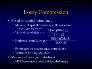
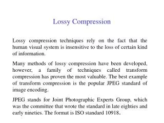
8.1 Introduction • • Lossless compression algorithms do not deliver compression ratios that are high enough. Hence, most multimedia compression algorithms are lossy. • • What is lossy compression? • – The compressed data is not the same as the original data, but a close approximation of it. • – Yields a much higher compression ratio than that of lossless compression. Li & Drew
8.2 Distortion Measures • • The three most commonly used distortion measures in image compression are: • – mean square error (MSE) σ2, • (8.1) • where xn, yn, and N are the input data sequence, reconstructed data sequence, and length of the data sequence respectively. • – signal to noise ratio (SNR), in decibel units (dB), • (8.2) • where is the average square value of the original data sequence and is the MSE. • – peak signal to noise ratio (PSNR), • (8.3) Li & Drew
8.3 The Rate-Distortion Theory • • Provides a framework for the study of tradeoffs between Rate and Distortion. • Fig. 8.1: Typical Rate Distortion Function. Li & Drew
8.4 Quantization • • Reduce the number of distinct output values to a much smaller set. • • Main source of the “loss” in lossy compression. • • Three different forms of quantization. • – Uniform: midrise and midtreadquantizers. • – Nonuniform: compandedquantizer. • – Vector Quantization. Li & Drew
Uniform Scalar Quantization • • A uniform scalar quantizer partitions the domain of input values into equally spaced intervals, except possibly at the two outer intervals. • – The output or reconstruction value corresponding to each interval is taken to be the midpoint of the interval. • – The length of each interval is referred to as the step size, denoted by the symbol Δ. • • Two types of uniform scalar quantizers: • – Midrise quantizers have even number of output levels. • – Midtreadquantizers have odd number of output levels, including zero as one of them (see Fig. 8.2). Li & Drew
• For the special case where Δ = 1, we can simply compute the output values for these quantizers as: • (8.4) • (8.5) • • Performance of an M level quantizer. Let B = {b0, b1, . . . , bM} be the set of decision boundaries and Y = {y1, y2, . . . , yM} be the set of reconstruction or output values. • • Suppose the input is uniformly distributed in the interval [−Xmax,Xmax]. The rate of the quantizer is: • (8.6) Li & Drew
Fig. 8.2: Uniform Scalar Quantizers: (a) Midrise, (b) Midtread. Li & Drew
Quantization Error of Uniformly Distributed Source • • Granular distortion: quantization error caused by the quantizer for bounded input. • – To get an overall figure for granular distortion, notice that decision boundaries bi for a midrise quantizer are [(i− 1)Δ, iΔ], i = 1..M/2, covering positive data X (and another half for negative X values). • – Output values yi are the midpoints iΔ−Δ/2, i= 1..M/2, again just considering the positive data. The total distortion is twice the sum over the positive data, or • (8.8) • • Since the reconstruction values yiare the midpoints of each interval, the quantization error must lie within the values [− , ]. For a uniformly distributed source, the graph of the quantization error is shown in Fig. 8.3. Li & Drew
Fig. 8.3: Quantization error of a uniformly distributed source. Li & Drew
Fig. 8.4: Companded quantization. • • Companded quantization is nonlinear. • • As shown above, a compander consists of a compressor function G, a uniform quantizer, and an expander function G−1. • • The two commonly used companders are the μ-law and A-law companders. Li & Drew
Vector Quantization (VQ) • • According to Shannon’s original work on information theory, any compression system performs better if it operates on vectors or groups of samples rather than individual symbols or samples. • • Form vectors of input samples by simply concatenating a number of consecutive samples into a single vector. • • Instead of single reconstruction values as in scalar quantization, in VQ code vectors with n components are used. A collection of these code vectors form the codebook. Li & Drew
8.5 Transform Coding • • The rationale behind transform coding: • If Y is the result of a linear transform T of the input vector X in such a way that the components of Y are much less correlated, then Y can be coded more efficiently than X. • • If most information is accurately described by the first few components of a transformed vector, then the remaining components can be coarsely quantized, or even set to zero, with little signal distortion. • • Discrete Cosine Transform (DCT) will be studied first. In addition, we will examine the Karhunen-Loève Transform (KLT) which optimallydecorrelates the components of the input X. Li & Drew
Spatial Frequency and DCT • • Spatial frequency indicates how many times pixel values change across an image block. • • The DCT formalizes this notion with a measure of how much the image contents change in correspondence to the number of cycles of a cosine wave per block. • • The role of the DCT is to decompose the original signal into its DC and AC components; the role of the IDCT is to reconstruct (re-compose) the signal. Li & Drew
Definition of DCT: • Given an input function f(i, j) over two integer variablesiand j (a piece of an image), the 2D DCT transforms it into a new function F(u, v), with integer u and v running over the same range as i and j. The general definition of the transform is: • (8.15) • where i, u = 0, 1, . . . ,M − 1; j, v = 0, 1, . . . ,N − 1; and the constants C(u) and C(v) are determined by • (8.16) Li & Drew
2D Discrete Cosine Transform (2D DCT): • (8.17) • where i, j, u, v = 0, 1, . . . , 7, and the constants C(u) and C(v) are determined by Eq. (8.5.16). • 2D Inverse Discrete Cosine Transform (2D IDCT): • The inverse function is almost the same, with the roles of f(i, j) and F(u, v) reversed, except that now C(u)C(v) must stand inside the sums: • (8.18) • where i, j, u, v = 0, 1, . . . , 7. Li & Drew
1D Discrete Cosine Transform (1D DCT): • (8.19) • where i = 0, 1, . . . , 7, u = 0, 1, . . . , 7. • 1D Inverse Discrete Cosine Transform (1D IDCT): • (8.20) • where i = 0, 1, . . . , 7, u = 0, 1, . . . , 7. Li & Drew
Fig. 8.6: The 1D DCT basis functions. Li & Drew
Fig. 8.7: Examples of 1D Discrete Cosine Transform: (a) A DC signal f1(i), (b) An AC signal f2(i). (a) (b) Li & Drew
Fig. 8.7 (cont’d): Examples of 1D Discrete Cosine Transform: (c) f3(i) = f1(i)+f2(i), and (d) an arbitrary signal f(i). (c) (d) Li & Drew
Fig. 8.8 An example of 1D IDCT. Li & Drew
The DCT is a linear transform: • In general, a transform T (or function) is linear, iff • (8.21) • where α and β are constants, p and q are any functions, variables or constants. • From the definition in Eq. 8.17 or 8.19, this property can readily be proven for the DCT because it uses only simple arithmetic operations. Li & Drew
The Cosine Basis Functions • • Function Bp(i) and Bq(i) are orthogonal, if • (8.22) • • Function Bp(i) and Bq(i) are orthonormal, if they are orthogonal and • (8.23) • • It can be shown that: Li & Drew
Fig. 8.9: Graphical Illustration of 8 × 8 2D DCT basis. Li & Drew
2D Separable Basis • • The 2D DCT can be separated into a sequence of two, 1D DCT steps: • (8.24) • (8.25) • • It is straightforward to see that this simple change saves • many arithmetic steps. The number of iterations required is reduced from 8 × 8 to 8+8. Li & Drew
Comparison of DCT and DFT • • The discrete cosine transform is a close counterpart to the Discrete Fourier Transform (DFT). DCT is a transform that only involves the real part of the DFT. • • For a continuous signal, we define the continuous Fourier transform F as follows: • (8.26) • Using Euler’s formula, we have • (8.27) • • Because the use of digital computers requires us to discretize the input signal, we define a DFT that operates on 8 samples of the input signal {f0, f1, . . . , f7} as: • (8.28) Li & Drew
Writing the sine and cosine terms explicitly, we have • (8.29) • • The formulation of the DCT that allows it to use only the cosine basis functions of the DFT is that we can cancel out the imaginary part of the DFT by making a symmetric copy of the original input signal. • • DCT of 8 input samples corresponds to DFT of the 16 samples made up of original 8 input samples and a symmetric copy of these, as shown in Fig. 8.10. Li & Drew
Fig. 8.10 Symmetric extension of the ramp function. Li & Drew
A Simple Comparison of DCT and DFT • Table 8.1 and Fig. 8.11 show the comparison of DCT and DFT on a ramp function, if only the first three terms are used. • Table 8.1 DCT and DFT coefficients of the ramp function Li & Drew
Fig. 8.11: Approximation of the ramp function: (a) 3 Term DCT Approximation, (b) 3 Term DFT Approximation. Li & Drew
Karhunen-Loève Transform (KLT) • • The Karhunen-Loève transform is a reversible linear transform that exploits the statistical properties of the vector representation. • • It optimally decorrelates the input signal. • • To understand the optimality of the KLT, consider the autocorrelation matrix RX of the input vector Xdefined as • (8.30) • (8.31) Li & Drew
• Our goal is to find a transform T such that the components of the output Y are uncorrelated, i.eE[YtYs] = 0, if t ≠ s. Thus, the autocorrelation matrix of Y takes on the form of a positive diagonal matrix. • • Since any autocorrelation matrix is symmetric and non-negative definite, there are k orthogonal eigenvectors u1, u2, . . . , uk and k corresponding real and nonnegative eigenvaluesλ1 ≥ λ2 ≥ ... ≥ λk ≥ 0. • • If we define the Karhunen-Loève transform as • (8.32) • • Then, the autocorrelation matrix of Ybecomes • (8.35) • (8.36) Li & Drew
KLT Example • To illustrate the mechanics of the KLT, consider the four 3D input vectors x1 = (4, 4, 5), • x2 = (3, 2, 5), x3 = (5, 7, 6), and x4 = (6, 7, 7). • • Estimate the mean: • • Estimate the autocorrelation matrix of the input: • (8.37) Li & Drew
• The eigenvalues of RX are λ1 = 6.1963, λ2 = 0.2147, and λ3 = 0.0264. The corresponding eigenvectors are • • The KLT is given by the matrix Li & Drew
• Subtracting the mean vector from each input vector and apply the KLT • • Since the rows of T are orthonormal vectors, the inverse transform is just the transpose: T−1 = TT , and • (8.38) • • In general, after the KLT most of the “energy” of the transform coefficients are concentrated within the first few components. This is the “energy compaction” property of the KLT. Li & Drew
8.6 Wavelet-Based Coding • • The objective of the wavelet transform is to decompose the input signal into components that are easier to deal with, have special interpretations, or have some components that can be thresholded away, for compression purposes. • • We want to be able to at least approximately reconstruct the original signal given these components. • • The basis functions of the wavelet transform are localized in both time and frequency. • • There are two types of wavelet transforms: the continuous wavelet transform (CWT) and the discrete wavelet transform (DWT). Li & Drew
The Continuous Wavelet Transform • • In general, a wavelet is a function ψ ∈ L2(R) with a zero average (the admissibility condition), • (8.49) • • Another way to state the admissibility condition is that the zeroth moment M0 of ψ(t) is zero. The pth moment is defined as • (8.50) • • The function ψ is normalized, i.e., ||ψ|| = 1 and centered at t = 0. A family of wavelet functions is obtained by scaling and translating the “mother wavelet” ψ • (8.51) Li & Drew
• The continuous wavelet transform (CWT) of f ∈ L2(R) at time u and scale s is defined as: • (8.52) • • The inverse of the continuous wavelet transform is: • (8.53) • where • (8.54) • and ψ(w) is the Fourier transform of ψ(t). Li & Drew
The Discrete Wavelet Transform • • Discrete wavelets are again formed from a mother wavelet, but with scale and shift in discrete steps. • • The DWT makes the connection between wavelets in the continuous time domain and “filter banks” in the discrete time domain in a multiresolution analysis framework. • • It is possible to show that the dilated and translated family of wavelets ψ • (8.55) • form an orthonormal basis of L2(R). Li & Drew
Multiresolution Analysis in the Wavelet Domain • • Multiresolution analysis provides the tool to adapt signal resolution to only relevant details for a particular task. • The approximation component is then recursively decomposed into approximation and detail at successively coarser scales. • • Wavelet functions ψ(t) are used to characterize detail information. The averaging (approximation) information is formally determined by a kind of dual to the mother wavelet, called the “scaling function” φ(t). • • Wavelets are set up such that the approximation at resolution 2−j contains all the necessary information to compute an approximation at coarser resolution 2−(j+1). Li & Drew
• The scaling function must satisfy the so-called dilation equation: • (8.56) • • The wavelet at the coarser level is also expressible as a sum of translated scaling functions: • (8.57) • (8.58) • • The vectors h0[n] and h1[n] are called the low-pass and high-pass analysis filters. To reconstruct the original input, an inverse operation is needed. The inverse filters are called synthesis filters. Li & Drew
Block Diagram of 1D Dyadic WaveletTransform • Fig. 8.18: The block diagram of the 1D dyadic wavelet transform. Li & Drew
Wavelet Transform Example • Suppose we are given the following input sequence. • {xn,i} = {10, 13, 25, 26, 29, 21, 7, 15} • • Consider the transform that replaces the original sequence with its pairwiseaveragexn−1,i and differencedn−1,i defined as follows: • • The averages and differences are applied only on consecutive pairs of input sequences whose first element has an even index. Therefore, the number of elements in each set {xn−1,i} and {dn−1,i} is exactly half of the number of elements in the original sequence. Li & Drew
• Form a new sequence having length equal to that of the original sequence by concatenating the two sequences {xn−1,i} and {dn−1,i}. The resulting sequence is • {xn−1,i, dn−1,i} = {11.5, 25.5, 25, 11,−1.5,−0.5, 4,−4} • • This sequence has exactly the same number of elements as the input sequence — the transform did not increase the amount of data. • • Since the first half of the above sequence contain averages from the original sequence, we can view it as a coarser approximation to the original signal. The second half of this sequence can be viewed as the details or approximation errors of the first half. Li & Drew
• It is easily verified that the original sequence can be reconstructed from the transformed sequence using the relations • xn, 2i= xn−1, i+ dn−1, i • xn, 2i+1 = xn−1,i− dn−1, i • • This transform is the discrete Haar wavelet transform. • Fig. 8.12: Haar Transform: (a) scaling function, (b) wavelet function. Li & Drew
Fig. 8.13: Input image for the 2D Haar Wavelet Transform. • (a) The pixel values. (b) Shown as an 8 × 8 image. Li & Drew
Fig. 8.14: Intermediate output of the 2D Haar Wavelet Transform. Li & Drew