Download
1 / 31
410 likes | 941 Views
Lossy Compression. Lossy compression techniques rely on the fact that the human visual system is insensitive to the loss of certain kind of information.

E N D
Lossy Compression Lossy compression techniques rely on the fact that the human visual system is insensitive to the loss of certain kind of information. Many methods of lossy compression have been developed, however, a family of techniques called transform compression has proven the most valuable. The best example of transform compression is the popular JPEG standard of image encoding. JPEG stands for Joint Photographic Experts Group, which was the committee that wrote the standard in late eighties and early nineties. The format is ISO standard 10918.
Transform coding Encoder performs four relatively straightforward operations: subimage decomposition, transformation, quantization and coding . Input image N x N Compressed image Construct n x n subimages Forward transform Quantizer Symbol encoder Decompressed image Symbol decoder Inverse transform Merge n x n subimages
Transform coding • map the image into a set of transform coefficients using a reversible, linear transform • a significant number of the coefficients will have small magnitudes • these can be coarsely quantized or discarded • compression is achieved during the quantization step, not during the transform
Block Coding • subdivide the image into small, non-overlapping blocks • apply the transform to each block separately • allows the compression to adapt to local image characteristics • reduces the computational requirements
Transform selection Consider an image f(x,y) of size N x N whose forward , discrete transform T(u,v) , can be expresses in terms of the general relation: (1) for u,v = 0, 1,…., n-1. . Given T(u,v),f(x,y) similarly can be obtained using the generalized inverse discrete transform: (2) for x,y = 0,1…., n-1 In these equations g(x,y,u,v) and h(x,y,u,v) are called the forward and inverse transform kernels, respectively. They also are referred to as basis functions or basic images. The T(u,v) for u=0,…n-1 are called transform coefficients.
Transform selection The forward and inverse transformation kernels in (1) and (2) determine the type of transform that is computed and overall computational complexity and reconstruction error of the transform coding system is which they are employed. The most well known transform kernel pair is (3) (4) where Subtracting these kernels into Eqs ( 1) and (2) yields a simplified version ( M=N) of the discrete Fourier transform pair . Using discrete Fourier transform of an n x n image we receive an array n x n of coefficients (5)
DCT is obtained by substituting the following ( equal ) kernels into (1) and (2) Discrete cosine transform (6) and similarly for (v) where Two dimensional discrete cosine conversion ( DCT ) is computed for each element ( one dimension for rows and one for columns), thus giving us 64 coefficients representing initial image frequencies. All these values are real, there is no complex mathematics here. Just as in Fourier analysis, each value in an 8 x 8 spectrum is the amplitude of a basis function. The first coefficient ( usually called DC is average of rest of 63 coefficients (AC). More important frequencies are grouped around upper left corner.
Hadamard transform • Many other orthogonal image transforms exist. • Hadamard, Paley, Walsh, Haar, Hadamard-Haar, Slant, discrete sine transform, wavelets, ... • The significance of image reconstruction from projections can be seen in computed tomography (CT), magnetic resonance imaging (MRI), positron emission tomography (PET), astronomy, holography, etc., where image formation is based on the Radon transform.
Transform selection • there are many that would work, including the discrete Fourier transform (DFT) • discrete cosine transform (DCT) has several advantages • real coefficients, rather than complex • packs more information into fewer coefficients than DFT • periodicity is 2N rather than N, reducing artifacts from discontinuities at block edges • discrete wavelet transform (DWT) is even better - JPEG 2000 use this - http://www.jpeg.org/JPEG2000.htm
Mean-square reconstruction error An n x n image f(x,y) can be expressed as a function of its 2D transform T(u,v) (7) for x, y = 0,1,…n-1 Since the inverse kernel h( x,y,u,v) depends only on the indices x, y ,u and v – not on the values of f(x,y) or T(u,v) - it can be viewed as defining a set of basis images. (8) (9)
Mean-square reconstruction error Then F, the matrix containing the pixels of the input subimage, is explicitly defined as a linear combination of n2 n x n matrices – that is , the Hu,v for u,v = 0,1,…n-1 of Eq(9). These matrices in fact are the basis images of the linear transform used to compute the series expansion weighting coefficients , T(u,v). If we define a transform coefficient masking function for u,v = 0,1,…n-1 , an approximation of F can be obtained from the truncated expansion: (10)
Mean-square reconstruction error The mean-square error between subimage F and approximation F’ then is Transformation that redistribute or pack the most information into the fewest coefficients provide the best subimage approximations and the smallest reconstruction errors. DCT provides a good compromise between information packing ability and computational complexity.
JPEG compression Considering there was no adequate standard for compressing 24-bit per pixel color data, committee came up with algorithm for compressing full color or greyscale images depicting real world scenes (like photographs). The main benefit JPEG exploits from human eye (in)sensitivity to certain image aspects and thus producing a powerful compression ratio even to 100:1 (usually 10:1 to 20:1 without noticeable degradation). The JPEG isn´t so good with line art, cartoons and one colored blocks. It is obvious that mentioned technique is lossy one, meaning that decompression won´t produce the original image to perfection, but a near match. The quality is left to user to selected it as he thinks it fit, having in mind preferred disk space / quality ratio.
JPEG compression • The algorithm is divided in four general steps and they are as follows : • Matrix creation and color scheme conversion • Discrete cosine conversion • Quantization • Additional encoding
JPEG compression • First , the image is divided into 8 x 8 blocks of pixels • Shift pixel values by substracting 128. The unsigned image values from the interval (0, 2b-1 ) are shifted to cover the interval ( -2b-1, 2b-1 –1) ( where 2b is a maximum number of grey level) • Compute a discrete cosine transform(DCT) of the block and generating an 8 x 8 block of coefficients . Since transforms like the DCT produce real numbers . Two dimensional discrete cosine conversion (DCT) is computed for each element (one dimension for rows and one for columns), thus giving us 64 DCT coefficients representing initial image frequencies. f(m,n) are pixel value and t(i,j) are frequencies coefficients.
40 0 20 0 0 0 15 0 0 0 0 0 0 0 0 0 47 0 25 0 5 0 9 0 0 0 0 0 0 0 0 0 22 0 0 0 11 0 0 0 0 0 0 0 0 0 0 0 2 0 12 0 16 0 4 0 0 0 0 0 0 0 0 0 JPEG compression The first coefficient (usually called DC) is average of rest of 63 coefficients (AC). More important frequencies are grouped around upper left corner. Another change is greater overall zero count (coefficient with value 0, see Figure.), which will contribute to the final compression ratio. So, step three produced 64 DCT coefficient matrix which follows us to another step ......
JPEG compression 4. One quatization table Q(u,v) is used to quatize the DCT coefficients A DCT coefficient T(u,v) is quantized by calculating : where u and v are spatial frequency parameters each ranging from 0 to 7, Q(u, v) is a value from a quatisation table and ‘”round” denotes rounding to the nearest integer. In fact, this approach implicitly discards components above a certain frequency by setting their coefficients to zero. The quantized DCT values are restricted to 11 bits.
JPEG compression 5. Arrange coefficients into a one-dimensional sequence by following a zigzag path from the lowest frequency component to the highest. This groups the zeros from the eliminated components into long runs. Lower frequencies coming first and higher last. Higher ones are likely to be zeroes and overall compression is improved. 6. Compress these runs if zeros by run-length encoding 7. The sequence is encoded by either Huffman or arithmetic encoding to form a final compressed file
JPEG compression See : http://http://www.jpeg.org/public/jpeghomepage.htm http://www.jpeg.org/JPEG2000.htm www.cs.sfu.ca/CourseCentral/365/li/interactive-jpeg/Ijpeg.html http://web.usxchange.net/elmo/jpeg.htm http://www.brycetech.com/tutor/windows/jpeg_compression.html http://www.cs.und.edu/~mschroed/jpeg.html
Compression of moving images MPEG is acronym for Moving Picture Expert Group, a group formed under ISO (International Organization for Standardization) and the IEC (International Electrotechnical Commission). Later, MPEG was given formal status within ISO/IEC. These three parts of the MPEG standard are: Part 1: System aspects Part 2: Video compression Part 3: Audio compression There are different types of MPEG. For example: MPEG-1, MPEG-2, MPEG-4 etc. The most important differences between them are data rate and applications. MPEG-1 has data rates on the order of 1.5 Mbit/s, MPEG-2 has 10 Mbit/s, and MPEG-4 has the lowest data rate of 64 Kbit/s.
MPEG - full-motion video compression • * Video and associated audio data can be compressed using MPEG compression algorithms. • * Using inter-frame compression, compression ratios of 200 can be achieved in full-motion, motion-intensive video applications maintaining reasonable quality. • * Currently, three standards are frequently cited: • MPEG-1 for compression of low-resolution (320x240) full-motion video at rates of 1-1.5 Mb/s • MPEG-2 for higher resolution standards like TV and HDTV at the rates of 2-80 Mb/s • MPEG-4 for small-frame full-motion compression with slow refresh needs, rates of 9-40kb/s for video-telephony and interactive multimedia like video-conferencing.
MPEG - full-motion video compression • MPEG compression facilitates the following features of the compressed video • random access, • fast forward/reverse searches, • reverse playback, • audio-visual synchronization, • robustness to error, • editability, • format flexibility, and • cost tradeoff
MPEG - full-motion video compression • The video data consist of a sequence of image frames. • In the MPEG compression scheme, three frame types are defined; • - intraframes I • - predicted frames P • forward, backward, or bi-directionally predicted or interpolated frames B
MPEG - full-motion video compression • Each frame type is coded using a different algorithm and Figure below shows how the frame types may be positioned in the sequence.
MPEG - full-motion video compression • I-frames are self-contained and coded using a DCT-based compression method similar to JPEG. • Thus, I-frames serve as random access frames in MPEG frame streams. • Consequently, I-frames are compressed with the lowest compression ratios. P-frames are coded using forward predictive coding with reference to the previous I- or P-frame and the compression ratio for P-frames is substantially higher than that for I-frames. • B-frames are coded using forward, backward, or bidirectional motion-compensated prediction or interpolation using two reference frames, closest past and future I- or P-frames, and offer the highest compression ratios.
MPEG - full-motion video compression • Note that in the hypothetical MPEG stream shown in Fig. 12.7, the frames must be transmitted in the following sequence (subscripts denote frame numbers): • I_1- P_4 - B_2 - B_3 - I_7 - B_5 - B_6 - etc. • the frames B_2 and B_3 must be transmitted after frame P_4 to enable frame interpolation used for B-frame decompression. • Clearly, the highest compression ratios can be achieved by incorporation of a large number of B-frames; if only I-frames are used, MJPEG compression results. • The following sequence seems to be effective for a large number of applications
MPEG - full-motion video compression • While coding the I-frames is straightforward, coding of P- and B-frames incorporates motion estimation. • For every 16x16 block of P- or B-frames, one motion vector is determined for P- and forward or backward predicted B-frames, two motion vectors are calculated for interpolated B-frames. • The motion estimation technique is not specified in the MPEG standard, however block matching techniques are widely used generally following the matching approaches.
MPEG - full-motion video compression • After the motion vectors are estimated, differences between the predicted and actual blocks are determined and represent the error terms which are encoded using DCT. • As usually, entropy encoding is employed as the final step. • MPEG-1 decoders are widely used in video-players for multimedia applications and on the World Wide Web. http://rnvs.informatik.tu-chemnitz.de/~jan/MPEG/HTML/mpeg_tech.html
MPEG-4 Natural Video Coding The MPEG-4 visual standard is developed to provide users a new level of interaction with visual contents. It provides technologies to view, access and manipulate objects rather than pixels, with great error robustness at a large range of bit rates. Application areas range from digital television, streaming video, to mobile multimedia and games. The MPEG-4 natural video standard consists of a collection of tools that support these application areas. The standard provides tools for shape coding, motion estimation and compensation, texture coding, error resilience, sprite coding and scalability. Conformance points in the form of object types, profiles and levels, provide the basis for interoperability
For next class Read paper MPEG-4 Natural Video Coding - An overview From : http://leonardo.telecomitalialab.com/icjfiles/mpeg-4_si/index.htm http://www.eecis.udel.edu/~amer/CISC651/651.html