Download
1 / 35
380 likes | 533 Views
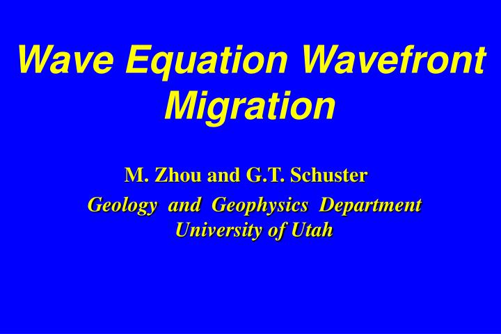
Wave Equation Wavefront Migration. M. Zhou and G.T. Schuster. Geology and Geophysics Department University of Utah. Outline. Objective Theory Examples SEG salt model Point-scatterer model Conclusions. Problem : Reverse-time migration accurate but

E N D
Wave Equation Wavefront Migration M. Zhou and G.T. Schuster Geology and Geophysics Department University of Utah
Outline • Objective • Theory • Examples • SEG salt model • Point-scatterer model • Conclusions
Problem:Reverse-time migration accurate but expensive Objective:Full-wave equation migration that is accurate but relatively efficient
Outline • Objective • Theory • Examples • SEG salt model • Point-scatterer model • Conclusions
Source field Reverse migrate data Theory Reverse-time migration: image
Theory WWM: Migration operator (focusing kernel) Data
shot geophone g (r’ | rs) g (rg | r’) Scatterer point r’ * Focusing kernel F(rs, r’, rg) = g (r’ | rs) g (rg | r’) Theory
shot geophone Reciprocity g (r’ | rs) g (rg | r’) g (r’ | rg) Scatterer point r’ * Focusing kernel F(rs, r’, rg) = g (r’ | rs) g (rg | r’) 1. Compute FocusingKernel by Src at Recs
shot geophone Reciprocity g (rs | r’) g (rg | r’) g (r’ | rs) Scatterer point r’ * Focusing kernel F(rs, r’, rg) = g (r’ | rs) g (rg | r’) 2. Compute Focusing Kernel by Src at Depth
Wavefront FD Modeling Wavefront FD Standard FD
Wavefront FD Modeling Wavefront FD Standard FD
Outline • Objective • Theory • Examples • SEG salt model • Wavefront forward modeling • Migration • Point-scatterer model • Conclusions
Wavefront FD Modeling X (km) X (km) 0 0 10 10 0 Depth (km) Standard Wavefront Time = 0.4
Wavefront FD Modeling X (km) X (km) 0 0 10 10 0 Depth (km) Standard Wavefront Time = 2 sec
Wavefront FD Modeling X (km) X (km) 0 0 10 10 0 Depth (km) Standard Wavefront Time = 4 s
Wavefront FD Modeling X (km) X (km) 6 6 8 8 0 Time (s) 5 Standard Wave Equation FD Wavefront (save 35% CPU time)
Wavefront FD Modeling X (km) X (km) 6 6 8 8 0 Time (s) 5 Data CSG200 Standard Wave Equation FD
Wavefront FD Modeling X (km) X (km) 6 6 8 8 0 Time (s) 5 Data CSG200 Wavefront
Outline • Objective • Theory • Examples • SEG salt model • Wavefront forward modeling • Migration • Point-scatterer model • Conclusions
Reverse-time Images X (km) 5 15 10 0 2.0 2.5 Depth (km) 3.0 3.5 Standard RTM Image 2.0 2.5 Depth (km) 3.0 3.5 Wavefront RTM Image (save 20% CPU time)
Reverse-time Images X (km) 5 15 10 0 2.0 2.5 Depth (km) 3.0 3.5 Standard RT Image 2.0 2.5 Depth (km) 3.0 3.5 Synthetic Model
Reverse-time Images X (km) 5 15 10 0 2.0 2.5 Depth (km) 3.0 3.5 Wavefront RT Image 2.0 2.5 Depth (km) 3.0 3.5 Synthetic Model
Reverse-time Images X (km) 8 6 12 10 2.0 2.5 Depth (km) 3.0 3.5 Standard RTM Image 2.0 2.5 Depth (km) 3.0 3.5 WWM Image
Reverse-time Images X (km) 8 6 12 10 2.0 2.5 Depth (km) 3.0 3.5 WWM Image 2.0 2.5 Depth (km) 3.0 3.5 Synthetic Model
Reverse-time Images X (km) 8 6 12 10 2.0 2.5 Depth (km) 3.0 3.5 Standard RTM Image 2.0 2.5 Depth (km) 3.0 3.5 Synthetic Model
Outline • Objective • Theory • Examples • SEG salt model • Point-scatterer model • Conclusions
shot geophone 0 Depth (km) scatterer 0.3 0.6 0 0.6 1.2 X (km) WWM + Incidence Angle
shot WWM + Incidence Angle 2t0 geophone t0 0 Depth (km) scatterer 0.3 0.6 0 0.6 1.2 X (km)
WWM + Incidence Angle X (km) 0 0.6 1.2 0.25 0.15 Time (s) 0.05 CSG gather
Focusing kernel CSG data geophone shot Scatterer point image point WWM + Incidence Angle
Focusing kernel CSG data geophone shot Scatterer point image point WWM + Incidence Angle
Focusing kernel CSG data geophone shot Scatterer point image point WWM + Incidence Angle
WWM + Incidence angle X (km) 0 0.6 1.2 0 Depth (km) 0.3 0.6 Standard Reverse-time Migration 0 Depth (km) 0.3 0.6 WWM + incidence angle
WWM + filtering constraints Wavefront forward modeling WWM by first arrivals Conclusions • reduce migration artifacts; • relatively efficient + accurate; • reduce artifacts; • high costs on I/O.
I am grateful for the financial • support from the members of • the 2001 UTAM consortium. • I am grateful for Yi Luo’s idea • on target-oriented wave equation • migration. Acknowledgements