Download
1 / 25
250 likes | 352 Views
Presentation of the Wave Equation Migration tool. 75th SEG Annual Meeting, Houston, TX. November 6 - 11, 2005. Long term R&D effort. 2D Paraxial propagator (Collino, 1989) Constrained least squares migration (Ehinger and Lailly, 1991; Duquet et al., 1994)

E N D
Presentation of the Wave Equation Migration tool 75th SEG Annual Meeting, Houston, TX. November 6 - 11, 2005.
Long term R&D effort • 2D Paraxial propagator (Collino, 1989) • Constrained least squares migration (Ehinger and Lailly, 1991; Duquet et al., 1994) • Common offset wavefield migration (Ehinger et al.; 1996) • 3D paraxial propagator (Collino and Joly, 1995) • 3D prestack wavefield migration (Duquet et al., 2001) • Comparison of 3D wavefield propagator (Lavaud and Duquet, 2001) • True amplitude wavefield migration (Joncour et al., 2005)
WE Method • Shot record Migration • Accurate • No assumption on the propagation complexity • No assumption on the acquisition geometry • Easy parallelization (shot, frequencies, ...) • Various One-Way propagation kernel • Finite Difference methods, Wavenumber methods, Mixed methods
One-Way propagation methods • Two main approaches : Finite Difference and Wavenumber • Finite difference (paraxial) : • Handle strong lateral velocity variations • Dip limited • Anisotropic Error in 3D (splitting method) • Wanenumber (SSF, PSPI) : • Handle gentle velocity variations • High dip accurate • Isotropic Error • Mixed method (FFD, Li) : • Combine both approaches
Accuracy of FD propagation 2 splitting directions 4 splitting directions 45 ° 68 °
One-Way propagation method • All these methods are implemented in our software namely: • SSF, PSPI, FD, FFD, LI, Optimized Li • FD propagation kernel: • 2 or 4 splitting directions • Unconditionally stable
Synthetic model Strong velocity contrasts + High dips Layer 1 = homogeneous velocity 1.5 km/s Layer 2 = layer 4 = lateral velocity gradient from 2 to 3 km/s Layer 3 = vertical velocity gradient from 3 to 4 km/s Layer 5 = homogeneous velocity 4 km/s
WE software • 2D/3D shot record migration • Common Angle Gather • Different parallelization level • Optimization strategy • Designed for huge size problem
Master Node Shot parallelization Slave Node n Slave Node 1 Frequency parallelization proc 1 proc 1 proc n proc n Two level parallelization
Two level parallelization • Coarse grain parallelization over shots • Masternode assign and send shared shots to each Slave node • Finer grain parallelization over frequency • Slavenode can be a dual/quadri processor or a cluster subset • mpi parallelization: each processor takes a subset of the frequencies • Reduced communication: • data reading + image condition
Optimization strategy • Shared shot allow to save cost associated with propagation matrix construction • Large step through water • Propagation depth step can be bigger than imaging depth step using an ad'hoc interpolation • ...
dz image=40m / dz propagation=40m 4 times faster
dz image=10m / dz propagation=40m+ ad'hoc interpolation 3 times faster
Designed for huge size problem • Memory requirement • Lateral propagation domain : 15km x 10km • Spatial sampling dx=dy=25m • Recording time= 10s • Frequency band = 40Hz (400 frequencies) • ~2 Gb core memory • Flexibility on the frequency range to be migrated
WE software • Shot record migration • accurate method • Fast and flexible algorithm • Various propagation kernels • handle high dips and strong velocity contrasts