Download
1 / 11
190 likes | 583 Views
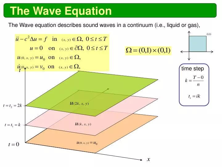
The Wave Equation. The Wave equation describes sound waves in a continuum (i.e., liquid or gas),. time step. Time Dependent Problem. Weak Formulation ( variational formulation). Fix a time t. Multiply equation (1) by and then integrate over the domain. Green’s theorem gives.

E N D
The Wave Equation The Wave equation describes sound waves in a continuum (i.e., liquid or gas), time step
Time Dependent Problem Weak Formulation ( variational formulation) Fix a time t Multiply equation (1) by and then integrate over the domain Green’s theorem gives
Variational Formulation Spatial Discretization
Spatial Discretization spatial semi-discretization equation Reduce into first order
Spatial Discretization spatial semi-discretization equation Reduce into first order
Spatial Discretization spatial semi-discretization equation Crank-Nicolson Method
Fully Discrete Equation Crank-Nicolson Method Crank-Nicolson Method (Matrix Form)
Computer Implementation % We solve the wave equation % d2u/dt2-div(grad(u))=0 on a square. % Problem definition g='squareg'; % The unit square b='squareb3'; % 0 on the left and right boundaries and % 0 normal derivative on the top & bottom. c=1; a=0; f=0; d=1; % pde coeff % Mesh [p,e,t]=initmesh('squareg'); % The initial conditions: % u(0)=atan(cos(pi/2*x)) and % dudt(0)=3*sin(pi*x).*exp(sin(pi/2*y)) x=p(1,:)'; y=p(2,:)'; u0=atan(cos(pi/2*x)); ut0=3*sin(pi*x).*exp(sin(pi/2*y)); % We want the sol at 31 pts in time between 0 and 5. n=401; tlist=linspace(0,5,n); % Solve hyperbolic problem uu=hyperbolic(u0,ut0,tlist,b,p,e,t,c,a,f,d); % To speed up plot, we interpolate to a rect grid. delta=-1:0.1:1; [uxy,tn,a2,a3]=tri2grid(p,t,uu(:,1),delta,delta); gp=[tn;a2;a3]; % Make the animation newplot; M=moviein(n); umax=max(max(uu)); umin=min(min(uu)); for i=1:n,... pdeplot(p,e,t,'xydata',uu(:,i),'zdata',... uu(:,i),'zstyle','continuous',... 'mesh','off','xygrid','on',... 'gridparam',gp,'colorbar','off');... axis([-1 1 -1 1 umin umax]); caxis([umin umax]); M(:,i)=getframe; end
T=0 100 time step 200 time step 400 time step