Download
1 / 32
330 likes | 351 Views
ENE 429 Antenna and Transmission Lines. Lecture 6 Power Gains and Stability Considerations of Two-Port Network. Power and power-gain expressions of a two-port network in a Z 0 system.

E N D
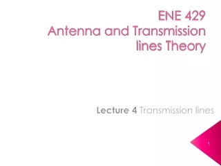
ENE 429Antenna and Transmission Lines Lecture 6Power Gains and Stability Considerations of Two-Port Network.
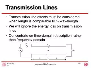
Power and power-gain expressions of a two-port network in a Z0 system • Power and power-gains are two main considerations in the design of a microwave transistor amplifier. To derive power and power-gains using traveling waves concept, we need to determine the reflection coefficients in the form of traveling waves and S parameters.
Reflection coefficient and traveling waves (1) • the source and the load reflection coefficient in a Z0 system are • For the transistor, the input and output traveling waves measured in a Z0 system are related by
Reflection coefficient and traveling waves (2) • The concepts of a reflection coefficient and traveling waves can be used even if there are no transmission lines at port 1 and port 2. • We can show that the input reflection coefficient
Reflection coefficient and traveling waves (3) • For the output reflection coefficient:
The power delivered to the input port of the transistor and can be shown in terms of S parameters as where and
The power available from the source (1) • The power available from the source is equal to the input power when IN = S* and can be expressed as • We can also express PIN in the form or PIN = PAVSMS
The power available from the source (2) where MS is the source mismatch factor which is equal to
The power delivered to the load ZL • The power delivered to the load ZL is and can be shown in terms of S parameters as where and
The power available from the network PAVN (1) • The power available from the network PAVN is equal to the power delivered to the load when L = OUT* and can be expressed as • We can also express PL in the form or PL = PAVNML
The power available from the network PAVN (2) where ML is the load mismatch factor which is equal to
There are 3 different power gains. (1) • The power gain GP is given by • The transducer power gain GT is given by
There are 3 different power gains. (2) Manipulating the denominator, GT can be also written in the form • The unilateral power gain GTU is an often employed approximation for the transducer power gain. GTU which neglects the feedback effect of the amplifier (S12 = 0) can be expressed as
There are 3 different power gains. (3) • The available power gain GA can be expressed in the form
Ex1 An RF amplifier has the following S-parameters: ,the input side of the amplifier is connected to a voltage source with E1 = 10 V and source impedance ZS = 50 . The output is connected to a load which also has an impedance ZL = 50 , given find the following quantities: a) transducer power gain GT, unilateral transducer gain GTU, available power gain GA, and operating power gain GP. b) power delivered to the load PL, power available from the source PAVS, and input power PIN.
Stability considerations • In a two-port network, oscillations are possible when either input or output port represents a negative resistance. This occurs when or • For a unilateral device (S12 = 0), the oscillations occur when or .
Unconditional stability • The two-port network is unconditionally stable if the real parts of ZIN and ZOUT are greater than zero for all passive load and source impedances. (1) (2) (3) (4) Note: all coefficients are normalized to the same characteristic impedance Z0.
Potential instability • This happens when some passive source and load terminations (some but not all values of S and L) produce input and output impedances having a negative real part.
Stability circles (1) • The graphical analysis is useful in the analysis of potentially unstable transistors. First, the regions where values of S and L produce and are determined, respectively. The solutions for S and L lie on circles (called stability circles) whose equations are given by and
Stability circles (2) • The radii and centers of the circles where and in the L plane and S plane, respectively, are obtained, namely L values for (Output Stability Circle): radius center
Stability circles (3) • S values for (Input Stability Circle): radius center where = S11S22-S12S21.
Stability circle construction in the Smith chart (a) L plane (b) S plane
Smith chart illustrating stable and unstable regions in the L plane. • The region where values of L (where ) produce are the stable regions.
Smith chart illustrating stable and unstable regions in the S plane. • The region where values of S (where ) produce are the stable regions.
Necessary and sufficient conditions for unconditional stability:(1) K > 1 where and . or K > 1 and
Necessary and sufficient conditions for unconditional stability:(2) • From practical point of view, most microwave transistors produced by manufacturers are either unconditionally stable or potentially unstable with 0< K < 1 and . Conditions for unconditionally stability for L plane and s plane.
Ex3 The S parameters of a BJT at VCE = 15 V and IC = 15 mA at f = 500 MHz, 1 GHz, 2 GHz, and 4 GHz are as follows: Determine the stability. If the transistor is potentially unstable at a given frequency, draw the input and output stability circles.
A potentially unstable transistor can be made unconditionally stable. • Even when the selection of S and L produces or , the circuit can be made stable if Re(ZS +ZIN) > 0 and Re(ZL+ZOUT) > 0 • A potentially unstable transistor can be made unconditionally stable by either resistively loading the transistor or by adding negative feedback. These techniques are not recommended in narrowband amplifiers.