REGRESSION WITH TIME SERIES VARIABLES

1. REGRESSION WITH TIME SERIES VARIABLES From Lecture Notes of Gary Koop, Heino Bohn Nielsen, Menelaos Karanasos, Kedem and Fokianos, and https://www.udel.edu/htr/Statistics/Notes816/class20.PDF,

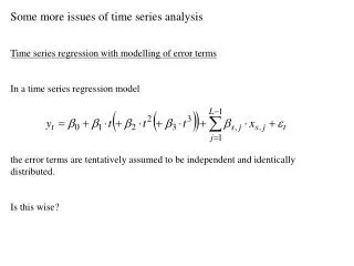
2. INTRODUCTION • The analysis of time series data is of vital interest to many groups, such as macroeconomists studying the behavior of national and international economies, finance economists who study the stock market, agricultural economists who want to predict supplies and demands for agricultural products. Climate related studies, forecasting energy demand, electricity prices, video processing, EEG signals, and so on. • Regression modelling goal is complicated when the researcher uses time series data since an explanatory variable may influence a dependent variable with a time lag. This often necessitates the inclusion of lags of the explanatory variable in the regression. • Lag: an interval of time between two related phenomena • Ytis a rv at time t and Yt-1 is a rv at time t-1. The lag between Ytand Yt-1 is 1. • If “time” is the unit of analysis we can still regress some dependent variable, Y, on one or more independent variables

3. INTRODUCTION Notation for time series data • Yt= value of Y in period t. • Data set: Y1,…,YT,T observations on the time series random variable Y • We consider only consecutive, evenly-spaced observations (for example, monthly, 1960 to 1999, no missing months) (missing and non-evenly spaced data introduce technical complications) • We will transform time series variables using lags and first differences • The j-th lag of a time series is: Yt-j • The first order difference of a time series: ΔYt=Yt-Yt-1 (it gives the change between periods t and t-1.)

4. INTRODUCTION • The correlation of a series with its own lagged values is called autocorrelation or serial correlation. • The first autocorrelation of Ytis corr(Yt,Yt–1) • The first autocovariance of Ytis cov(Yt,Yt–1) Population: Sample:

5. INTRODUCTION • The partial autocorrelation function (PACF) is the correlation between Yt and Yt-k after their mutual linear dependency on the intervening variables Yt-1, Yt-2, …, Yt-k+1has been removed. • The conditional correlation is usually referred as the partial autocorrelation in time series. ACF and PACF are very important tools in time series analysis to be able to understand the relationship between Yt and Yt-k.

6. INTRODUCTION • Since we have only one observation for each r.v. Yt, inference is too complicated if distributions (or moments) change for all t (i.e. change over time). So, we need a simplification. r.v.

7. INTRODUCTION • To be able to identify the structure of the series, we need the joint pdf of Y1, Y2,…, Yn. However, we have only one sample. That is, one observation from each random variable. Therefore, it is very difficult to identify the joint distribution. Hence, we need an assumption to simplify our problem. This simplifying assumption is known as STATIONARITY.

8. INTRODUCTION • The stationarity is the most vital and common assumption in time series analysis. • The basic idea of stationarity is that the probability laws governing the process do not change with time. • WEAK (COVARIANCE) STATIONARITY OR STATIONARITY IN WIDE SENSE: A time series is said to be stationary if its first and second order moments are unaffected by a change of time origin.

9. INTRODUCTION • A process {at} is called a white noise (WN) process, if it is a sequence of uncorrelated random variables from a fixed distribution with constant mean {E(at)=}, constant variance{Var(at)= } and Cov(Yt, Yt-k)=0 for all k≠0. • It is a stationary process with autocovariance function Basic Phenomenon: ACF=PACF=0, k0.

10. FIRST ORDER AUTOREGRESSIVE MODEL • A simple model for Ytgiven the past is the autoregressive model • Here,  is the process mean. • The AR(1) model can be estimated by OLS regression of Ytagainst Yt–1

11. NON-STATIONARITY • Non-stationarity is tested by unit root test. • The most popular unit root tests are Augmented Dickey Fuller (ADF) and Phillips-Perron (PP) tests. • H0: unit root exists, i.e., the series is non-stationary H1: stationary • If we cannot reject the null hypothesis, usually we apply differencing to the series and work with the differenced series, i.e., ΔYt=Yt-Yt-1

12. EXAMPLE • Consider the time series plot, ACF and PACF plots a series > pp.test(y) Phillips-Perron Unit Root Test data: y Dickey-Fuller Z(alpha) = -11.1817, Truncation lag parameter = 4, p-value = 0.4673 alternative hypothesis: stationary

13. EXAMPLE • After applying the first order difference • > pp.test(ydif) • Phillips-PerronUnit Root Test • data: ydif • Dickey-Fuller Z(alpha) = -97.7996, Truncation lag parameter = 3, • p-value = 0.01 • alternative hypothesis: stationary • After the first order difference, the series became stationary. We don’t need the second difference.

14. REGRESSION WITH TIME SERIES VARIABLES

15. REGRESSION WITH TIME SERIES VARIABLES Main Assumption: • Consider a time series yt and the k × 1 vector time series xt. We assume (1) that zt = (yt, x’t)’ has a joint stationary distribution; and (2) that the process ztis weakly dependent, so that zt and zt+kbecomes approximately independent for k → ∞.

16. INTRODUCTION

17. Autoregressive Errors • Consider the case where the errors are truly autoregressive: • If ρ is known we can write • The GLS model is subject to a so-called common factor restriction: three regressors but only two parameters, ρ and β. Estimation is non-linear. • Residual autocorrelation indicates that the model is not dynamically complete

18. Test for No-Autocorrelation • The Durbin Watson (DW) test is derived for finite samples. Based on strict exogeneity. Not valid in many models.

19. SOME REGRESSION MODELS WHEN VARIABLES ARE TIME SERIES

20. STATIC MODEL • A contemporaneous relation between y and z can be captured by a static model: yt = β0 + β1zt + ut , t = 1, 2, . . . , n. When to use? Change in z at time t have immediate effect on y: ∆yt = β1∆zt , when ∆ut = 0. We would like to know tradeoff between y and z.

21. (FINITE) DISTRIBUTED LAG MODEL • We allow one or more variables to affect y with a lag. yt= α0 + δ0zt + δ1zt−1 + δ2zt−2 +… δqzt−q + ut , where δ0 is so-called “impact propensity” or “impact multiplier” and it reflects immediate change in y. • For a temporary, 1-period change, y returns to its original level in period q + 1 • We can call δ0 + δ1 + . . . + δq the ‘long-run propensity” (LRP) and it reflects the long-run change in y after a permanent change

22. AUTOREGRESSIVE DISTRIBUTED LAG (ADL) MODEL • Augment AR(p) with lags of explanatory variables produces ADL model • p lags of Y, q lags of X ⇒ ADL(p,q). Note: X and Y must have the same stationarity properties (either must both be stationary or both have a unit root). If not use:

23. AUTOREGRESSIVE DISTRIBUTED LAG (ADL) MODEL • Estimation and interpretation of the ADL(p,q) model depends on whether Y and X are stationary or have unit roots. • Before you estimate an ADL model you should test both Y and X for unit roots using the Dickey-Fuller test.

24. MULTICOLLINEARITY • This form of ADL model less likely to run into multicollinearityproblems. • One thing researchers often calculate is the long run or total multiplier • Suppose that X and Y are in an equilibrium or steady state. Then X rises (permanently) by one unit, affecting Y, which starts to change, settling down in the long run to a new equilibrium value. • Difference between old and new equilibrium values for Y is long run effect of X on Y and called long run multiplier. This multiplier is often of great interest for policy makers who want to know the eventual effects of their policy changes in various areas. • For ADL(p; q) model long run multiplier is: -/

25. ADL in R

26. ADL in R • Illustration: Different specifications of consumption function taken fromGreene(2003). • Data: Quarterly US macroeconomic data from 1950(1) – 2000(4) provided by USMacroG, a “ts” time series. Contains disposable income dpi and consumption (in billion USD). • Visualization: Employ corresponding plot() method. R> data("USMacroG", package = "AER") R> plot(USMacroG[, c("dpi", "consumption")], lty = c(3, 1), + lwd = 2, plot.type = "single", ylab = "") R> legend("topleft", legend = c("income", "consumption"), + lwd = 2, lty = c(3, 1), bty = "n")

33. TIME SERIES REGRESSION WHEN X AND Y ARE STATIONARY • Minimal changes (e.g. OLS fine, testing done in standard way, etc.), except for the interpretation of results. • Lag lengths, p and q can be selected using sequential tests. • It is convenient to rewrite ADL model as:

34. TIME SERIES REGRESSION WHEN X AND Y ARE STATIONARY • Effect of a slight change in X on Y in the long run. • To understand the long run multiplier: • Suppose X and Y are in an equilibrium or steady state. All of a sudden, X changes slightly. This affects Y, which will change and, in the long run, move to a new equilibrium value. • The difference between the old and new equilibrium values for Y = the long run multiplier effect of X on Y. • Can show that the long-run multiplier is −θ/. • For system to be stable (a concept we will not formally define), we need  <0.

35. EXAMPLE: THE EFFECT OF FINANCIAL LIBERALIZATION ON ECONOMIC GROWTH • Time series data for 98 quarters for a country • Y = the percentage change in GDP • X = the percentage change in total stock market capitalization • Assume Y and X are stationary

36. EXAMPLE: THE EFFECT OF FINANCIAL LIBERALIZATION ON ECONOMIC GROWTH • ADL(2,2) with Deterministic Trend Model

37. EXAMPLE: THE EFFECT OF FINANCIAL LIBERALIZATION ON ECONOMIC GROWTH • Estimate of long run multiplier: −(0.125/−0.120)=1.042 • Remember that the dependent and explanatory variables are % changes: • The long run multiplier effect of financial liberalization on GDP growth is 1.042 percent. • If X permanently increases by one percent, the equilibrium value of Y will increase by 1.042 percent.

38. TIME SERIES REGRESSION WHEN Y AND X HAVE UNIT ROOTS: SPURIOUS REGRESSION • Now assume that Y and X have unit roots. • Consider the standard regression of Y on X: • OLS estimation of this regression can yield results which are completely wrong. • These problems carry over to the ADL model.

39. TIME SERIES REGRESSION WHEN Y AND X HAVE UNIT ROOTS: SPURIOUS REGRESSION • Even if the true value of β is 0, OLS can yield an estimate, , which is very different from zero. βˆ • Statistical tests (using the t-stat or P-value) may indicate that β is not zero. • If β=0, then the R2 should be zero. In the present case, the R2 will often be quite large. • This is called the spurious regression problem. • Practical Implication: • With the one exception that we note below, you should never run a regression of Y on X if the variables have unit roots. • The exception occurs if Y and X are cointegrated.

40. HETEROSCESDASTICITY • Gauss–Markov assumptions start with the assumption of homoskedasticity. • Under heteroskedasticity, • OLS is still unbiased. • OLS is no longer efficient. • OLS e.s.e.’s are incorrect, so C.I.,t-, and F- statistics are incorrect. • Under heteroskedasticity,

41. HETEROSCESDASTICITY • We can use squared residuals to test for heteroskedasticity. • In the White test, we regress the squared residuals against all explanators, squares of explanators, and interactions of explanators. The nR2 of the auxilliary equation is distributed Chi-squared. • The Breusch–Pagan test is similar, but the econometrician chooses the explanators for the auxilliary equation.

42. HETEROSCESDASTICITY • Under heteroskedasticity, the BLUE Estimator is Generalized Least Squares. • To implement GLS: • Divide all variables by di • Perform OLS on the transformed variables. • If we have used the correct di , the transformed data are homoskedastic.

43. HETEROSCESDASTICITY • For example, consider the relationship • We are concerned that Var(ei) may vary with income. • We need to make an assumption about how Var(ei) varies with income. • An initial guess: • di = incomei • If we have modeled heteroskedasticity correctly, then the BLUE Estimator is

44. HETEROSCESDASTICITY • If we have the correct model of heteroskedasticity, then OLS with the transformed data should be homoskedastic. • Using a White test, we reject the null hypothesis of homoskedasticity of the model with transformed data. • Our first guess didn’t work very well. • Let’s try

45. Feasible GLS • This time, we fail to reject the null hypothesis of homoskedasticity. • We usually do NOT know di, so GLS is infeasible. • We can, however, ESTIMATE di • We call GLS with estimates of di“Feasible Generalized Least Squares.” • To begin, we need to assume some model for the heteroskedasticity. • Then we estimate the parameter/s of the model.

46. Feasible GLS • One reasonable model for the error terms could be that the variance is proportional to some power of the explanator. • For example, in the rent-income example, we tried both

47. Feasible GLS • To implement FGLS, we have assumed • To estimate this equation using linear regression methods, we can take advantage of the properties of logs: • Regress

48. Feasible GLS • Estimate the regression with OLS. • Regress • Divide every variable by: • Apply OLS to the transformed data. • FGLS is not a mechanistic procedure. • Applying FGLS to the rent-income example, our estimated h value is 1.21 • We should divide all our variables by incomei0.605. This is very close to dividing by the square root of income, as we did in the second part of the example.

49. FGLS EXAMPLE

50. White Robust Standard Errors • If we know the exact nature of the heteroskedasticity (i.e. if we know the di), then they can simply divide all variables by di and apply GLS. • If the diare unknown, but we are willing to make some assumptions about their functional form, then the di can be estimated by FGLS. • If we are unwilling to make assumptions about the nature of the heteroskedasticity, we can implement OLS to get unbiased, but inefficient, estimates. • Then we must correct the estimated standard errors using White Robust Standard Errors.