REGRESSION WITH TIME SERIES VARIABLES

REGRESSION WITH TIME SERIES VARIABLES

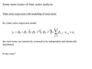
INTRODUCTION • Regression modelling goal is complicated when the researcher uses time series data since an explanatory variable may influence a dependent variable with a time lag. This often necessitates the inclusion of lags of the explanatory variable in the regression. • If “time” is the unit of analysis we can still regress some dependent variable, Y, on one or more independent variables

INTRODUCTION

INTRODUCTION E( )

SOME REGRESSION MODELS WHEN VARIABLES ARE TIME SERIES (Also referred to as the ARDL or ARX model)

STATIC MODEL (Levels Model)

AUTOREGRESSIVE DISTRIBUTED LAG (ADL) MODEL

AUTOREGRESSIVE DISTRIBUTED LAG (ADL) MODEL • Estimation and interpretation of the ADL(p,q) model depends on whether Y and X are stationary or have unit roots. • Before you estimate an ADL model you should test both Y and X for unit roots using the Augmented Dickey-Fuller (ADF) test.

TIME SERIES REGRESSION WHEN X AND Y ARE STATIONARY • Minimal changes (e.g. OLS fine, testing done in standard way, etc.), except for the interpretation of results. • Lag lengths, p and q can be selected using sequential tests. • It is convenient to rewrite ADL model as:

TIME SERIES REGRESSION WHEN X AND Y ARE STATIONARY • Effect of a slight change in X on Y in the long run. • To understand the long run multiplier: • Suppose X and Y are in an equilibrium or steady state. • All of a sudden, X changes slightly. • This affects Y, which will change and, in the long run, move to a new equilibrium value. • The difference between the old and new equilibrium values for Y = the long run multiplier effect of X on Y. • Can show that the long-run multiplier is −θ/φ. • For system to be stable (a concept we will not formally define), we need φ < 0.

EXAMPLE: THE EFFECT OF FINANCIAL LIBERALIZATION ON ECONOMIC GROWTH

EXAMPLE: THE EFFECT OF FINANCIAL LIBERALIZATION ON ECONOMIC GROWTH • Time series data for 98 quarters for a country • Y = the percentage change in GDP • X = the percentage change in total stock market capitalization • Assume Y and X are stationary (*this is not a necessary condition to utilize the ADL model as we know the ADL model is suitable for all I(0), all I(1) and, mixed I(0) and I(1). It is a very flexible model indeed.)

EXAMPLE: THE EFFECT OF FINANCIAL LIBERALIZATION ON ECONOMIC GROWTH • ADL(2,2) with Deterministic Trend Model

EXAMPLE: THE EFFECT OF FINANCIAL LIBERALIZATION ON ECONOMIC GROWTH • Estimate of long run multiplier: −(0.125/−0.120)=1.042 • Remember that the dependent and explanatory variables are % changes: • The long run multiplier effect of financial liberalization on GDP growth is 1.042 percent. • If X permanently increases by one percent, the equilibrium value of Y will increase by 1.042 percent.

TIME SERIES REGRESSION WHEN Y AND X HAVE UNIT ROOTS: SPURIOUS REGRESSION

SPURIOUS REGRESSION Set-up: Regress What do you expect to get?

SpuriousRegression (continued) What happened really

SpuriousRegression (continued) Spurious Regression Problem: Regression of an integrated series on another unrelated integrated series produces t-ratios on the slope parameter which indicates a relationship much more often than they should at the nominal test level. This problem does not dissapear as the sample size is increased. In a Spurious Regression the errors would be correlated and the standard t-statistic will be wrongly calculated because the variance of the errors is not consistently estimated. In the I(0) case the solution is:

SpuriousRegression (continued)

SpuriousRegression (continued) Does it make sense to preform a regression between two I(1) variables? Yes if the regression error is I(0). Can this be possible? The same question was asked by David Hendry to Clive Granger some time ago. Clive answered NO WAY!!!!! but he also said that he would think about. In the plane trip back home to San Diego, Clive thought about it and concluded that YES IT IS POSSIBLE. It is possible when both variables share the same source of the I(1)’ness (co-I(1)), that is, when both variables move together in the long-run (co-move), ... That is, when both variables are COINTEGRATED!

Cointegration, Example 1

Cointegration, Example 2 Theory of Purchasing Power Parity (PPP) “Apart from transportation costs, good should sell for the same effective price in two countries” An index of the price level in the USA $ per £ Price Index for UK In logs : A weaker version of the PPP: If the three variables are I(1) and zt is I(0) then the PPP theory is implying cointegrating between pt, st and p*t .

They shared the Nobel Prize in Economic s in 2003 for developing the ARCH model (Engle) and Cointegration (Granger) Robert F. Engle (born in 1942) American economist, currently teaches at New York University, Stern School of Business Clive Granger (1934 – 2009) British economist, taught at University of Nottinghan in Britain & University of California, San Diego in US

Test forCointegration, theEngle-Granger Test

EG test • R: fit5 = egcm(x,y) • SAS: procAUTOREG; model y = x/ nlag=1stationarity =(adf=1);

The Error Correction Model (ECM) When two I(1) series are co-integrated, the best regression model between the two is the error correction model as it features both their long-run relationship, as well as their short-term relationship.

Relationship between the Error Correction Model (ECM) and the Autoregressive Distributed Lag (ADL) Model

Further Comparison of the Error Correction Model (ECM) and the Autoregressive Distributed Lag (ADL) Model • The ECM model enjoys a clear interpretation by linking incorporating • both the short term relationship and the long term relationship in the same • regression model. • While the ECM model is designed when all variables are I(1), the ADL • Model is applicable when (1) all variables are I(1) , and (2) when we have a • mixture of I(1) and I(0) variables.

To be continued … for more complicated scenarios such as more regressors and more cointegration relationships.

REGRESSION WITH TIME SERIES VARIABLES