Download
1 / 26
260 likes | 388 Views
Linear optics from closed orbits (LOCO). Given linear optics (quad. gradients), can calculate response matrix. Reverse is possible – calculate gradients from measured response matrix.

E N D
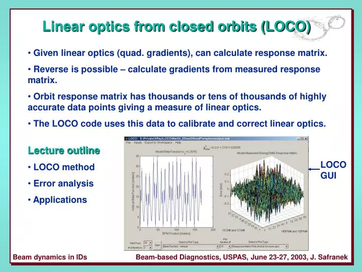
Linear optics from closed orbits (LOCO) • Given linear optics (quad. gradients), can calculate response matrix. • Reverse is possible – calculate gradients from measured response matrix. • Orbit response matrix has thousands or tens of thousands of highly accurate data points giving a measure of linear optics. • The LOCO code uses this data to calibrate and correct linear optics. • Lecture outline • LOCO method • Error analysis • Applications LOCO GUI Beam-based Diagnostics, USPAS, June 23-27, 2003, J. Safranek
NSLS VUV ring example • The VUV ring optics were not well controlled. There was a problem with incorrect compensation for insertion device (ID) focusing. LOCO was used to calibrate the strength of the ID focusing and to find the changes the current to the quadrupoles that best restored the optics. • The results were • 20% increase in lifetime • Few percent decrease in both ex and ey IDs Beam-based Diagnostics, USPAS, June 23-27, 2003, J. Safranek
Method The orbit response matrix is defined as The parameters in a computer model of a storage ring are varied to minimize the c2 deviation between the model and measured orbit response matrices (Mmod and Mmeas). The si are the measured noise levels for the BPMs; E is the error vector. The c2 minimization is achieved by iteratively solving the linear equation For the changes in the model parameters, Kl, that minimize ||E||2=c2. Beam-based Diagnostics, USPAS, June 23-27, 2003, J. Safranek
Response matrix review The response matrix is the shift in orbit at each BPM for a change in strength of each steering magnet. Vertical response matrix, BPM i, steerer j: Horizontal response matrix: Additional h term keeps the path length constant (fixed rf frequency). LOCO option to use this linear form of the response matrix (faster) or can calculate response matrix including magnet nonlinearities and skew gradients (slower, more precise). First converge with linear response matrix, then use full response matrix. Beam-based Diagnostics, USPAS, June 23-27, 2003, J. Safranek
Parameters varied to fit the orbit response matrix NSLS XRay Ring fit parameters: 56 quadrupole gradients 48 BPM gains, horizontal 48 BPM gains, vertical 90 steering magnet kicks =242 Total fit parameters NSLS XRay data: (48 BPMs)*(90 steering magnets) =4320 data points c2 fit becomes a minimization problem of a function of 242 variables. Fit converted to linear algebra problem, minimize ||E||2=c2. For larger rings, fit thousands of parameters to tens of thousands of data points. For rings the size of LEP, problem gets too large to solve all at once on existing computers. Need to divide ring into sections and analyze sections separately. Beam-based Diagnostics, USPAS, June 23-27, 2003, J. Safranek
More fit parameters • Why add BPM gains and steering magnet calibrations? • Adding more fit parameters increases error bars on fit gradients due to propagation of random measurement noise on BPMs. If you knew that all the BPMs were perfectly calibrated, it would be better not to vary the BPM gains in the fit. • More fit parameters decreases error on fit gradients from systematic modeling errors. Not varying BPM gains introduces systematic error. • As a rule, vary parameters that introduce ‘significant’ systematic error. This usually includes BPM gains and steering magnet kicks. • Other parameters to vary: • Quadrupole roll (skew gradient) • Steering magnet roll • BPM coupling • Steering magnet energy shifts • Steering magnet longitudinal centers } Parameters for coupled response matrix, Beam-based Diagnostics, USPAS, June 23-27, 2003, J. Safranek
Fitting energy shifts. Horizontal response matrix: Betatron amplitudes and phases depend only on storage ring gradients: Dispersion depends both on gradients and dipole field distribution: If the goal is to find the gradient errors, then fitting the full response matrix, including the term with h, will be subject to systematic errors associated with dipole errors in the real ring not included in the model. This problem can be circumvented by using a “fixed momentum” model, and adding a term to the model proportional to the measured dispersion is a fit parameter for each steering magnet. In this way the hmodel is eliminated from the fit, along with systematic error from differences between hmodel and hmeas. Beam-based Diagnostics, USPAS, June 23-27, 2003, J. Safranek
Finding gradient errors at ALS • LOCO fit indicated gradient errors in ALS QD magnets making by distortion. • Gradient errors subsequently confirmed with current measurements. • LOCO used to fix by periodicity. • Operational improvement (Thursday lecture). Beam-based Diagnostics, USPAS, June 23-27, 2003, J. Safranek
Different goals when applying LOCO • There are a variety of results that can be achieved with LOCO: • Finding actual gradient errors. • Finding changes in gradients to correct betas. • Finding changes in gradients to correct betas and dispersion. • Finding changes in local gradients to correct ID focusing (Thursday’s lecture). • Finding changes in skew gradients to correct coupling and hy (Wednesday’s lecture). • Finding transverse impedance (Friday’s lecture). The details of how to set up LOCO and the way the response matrix is measured differs depending on the goal. In the previous example for the ALS, the goals were 1 and 2. LOCO is set up differently for each. Beam-based Diagnostics, USPAS, June 23-27, 2003, J. Safranek
Finding gradient errors • If possible, measure two response matrices – one with sextupoles off and one with sextupoles on. • Fit the first to find individual quadrupole gradients. • Fit the second to find gradients in sextupoles. • Fewer gradients are fit to each response matrix, increasing the accuracy. • … Measure a 3rd response matrix with IDs closed. • Vary all quadrupole gradients individually (maybe leave dipole gradient as a family). • Use either 1.) fixed-momentum response matrix and fit energy shifts or 2.) fixed-path-length depending on how well 1/r in the model agrees with 1/r in the ring (i.e. how well is the orbit known and controlled). • Get the model parameters to agree as best as possible with the real ring: model dipole field roll-off; check longitudinal positions of BPMs and steering magnets; compensate for known nonlinearities in BPMs. • Add more fitting parameters if necessary to reduce systematic error (for example, fit steering magnet longitudinal centers in X-Ray Ring.) Beam-based Diagnostics, USPAS, June 23-27, 2003, J. Safranek
Correcting betas and dispersion • Measure response matrix with ring in configuration for delivered beam. • Sextupoles on • Correct to golden orbit • IDs closed (depending on how you want to deal with ID focusing) • Fit only gradients that can be adjusted in real ring. • Do not fit gradients in sextupoles or ID gradients • If a family of quadrupoles is in a string with a single power supply, constrain the gradients of the family to be the same. • To correct betas only, use fixed-momentum model matrix and fit energy shifts, so dispersion is excluded from fit. • To correct betas and dispersion, use fixed-path length matrix and can use option of including h as an additional column in response matrix. • To implement correction, change quadrupole current of nth quadrupole or quad family: Beam-based Diagnostics, USPAS, June 23-27, 2003, J. Safranek
Correcting betas in PEPII Often times, finding the quad changes required to correct the optics is easier than finding the exact source of all the gradient errors. For example, in PEPII there are not enough BPMs to constrain a fit for each individual quadrupole gradient. The optics still could be corrected by fitting quadrupole families. Independent bmeasurements confirmed that LOCO had found the real b’s(x2.5 error!) Quadrupole current changes according to fit gradients restored ring optics to the design. PEPII HER by,design PEPII HER by,LOCO fit Beam-based Diagnostics, USPAS, June 23-27, 2003, J. Safranek
Skip? Beam-based Diagnostics, USPAS, June 23-27, 2003, J. Safranek
LOCO GUI fitting options menu Remove bad BPMs or steerers from fit. Include coupling terms (Mxy, Myx) Model response matrix: linear or full non-linear; fixed-momentum or fixed-path-length Include h as extra column of M Let program choose Ds when calculating numerical derivatives of M with quadrupole gradients. More on these coming. Reject outlier data points. Beam-based Diagnostics, USPAS, June 23-27, 2003, J. Safranek
Error bars from BPM measurement noise LOCO calculates the error bars on the fit parameters according to the measured noise levels of the BPMs. LOCO uses singular value decomposition (SVD) to invert and solve for fit parameters. The results from SVD are useful in calculating and understanding the error bars. SVD reduces the matrix to a sum of a product of eigenvectors of parameter changes, v, times eigenvectors, u, which give the changes in the error vector, E, corresponding to v. The singular values, wl, give a measure of how much a change of parameters in the direction of v in the multidimensional parameter space changes the error vector. (For a more detailed discussion see Numerical Recipes, Cambridge Press.) Beam-based Diagnostics, USPAS, June 23-27, 2003, J. Safranek
SVD and error bars A small singular value, wl, means changes of fit parameters in the direction vl make very little change in the error vector. The measured data does not constrain the fit parameters well in the direction of vl; there is relatively large uncertainty in the fit parameters in the direction of vl. The uncertainty in fit parameter Kl is given by Illustration for 2 parameter fit: K2 Together the vl and wl pairs define an ellipse of variances and covariances in parameter space. LOCO converges to the center of the ellipse. Any model within the ellipse fits the data as well, within the BPM noise error bars. best fit model Ellipse around other models that also give good fit. K1 Beam-based Diagnostics, USPAS, June 23-27, 2003, J. Safranek
SVD and error bars, II Eigenvectors with small singular values indicate a direction in parameter space for which the measured data does not constrain well the fit parameters. The two small singular values in this example are associated with a degeneracy between fit BPM gains and steering magnet kicks. If all BPM gains are increased and kicks decreased by a single factor, the response matrix does not change. There two small singular values – horizontal and vertical plane. This problem can be eliminated by including coupling terms in the fit and including the dispersion as a column of the response matrix (without fitting the rf frequency change). Singular value spectrum; green circles means included in fit; red X means excluded. 2 small singular values plot of 2 v with small w eigenvector, v BPM Gx BPM Gy qx qy energy shifts & K’s Beam-based Diagnostics, USPAS, June 23-27, 2003, J. Safranek
SVD and error bars, III LOCO throws out the small singular values when inverting and when calculating error bars. This results in small error bars calculated for BPM gains and steering magnet kicks. The error bars should be interpreted as the error in the relative gain of one BPM compared to the next. The error in absolute gain is much greater. If other small singular values arise in a fit, they need to be understood. small error bars vertical BPM gain vertical BPM number Beam-based Diagnostics, USPAS, June 23-27, 2003, J. Safranek
Analyzing multiple data sets Analyzing multiple data sets provides a second method for investigating the variation in fit parameters from measurement noise. The results shown here are for the NSLS X-Ray ring, and are in agreement with the error bars calculated from analytical propagation of errors. Beam-based Diagnostics, USPAS, June 23-27, 2003, J. Safranek
Systematic error • The error in fit parameters from systematic differences between the model and real rings is difficult to quantify. • Typical sources of systematic error are: • Magnet model limitations – unknown multipoles; end field effects. • Errors in the longitudinal positions of BPMs and steering magnets. • Nonlinearities in BPMs. • electronic and mechanical • avoid by keeping kick size small. Fit dominated by systematics from BPM nonlinearity Fit dominated by BPM noise Increasing steering kick size Beam-based Diagnostics, USPAS, June 23-27, 2003, J. Safranek
Systematic error, II Error vector histogram With no systematic errors, the fit should converge to Number of points (8640 total) N = # of data points M = # of fit parameters This plot shows results with simulated data with With real data the best fit I’ve had is fitting NSLS XRay ring data to 1.2 mm for 1.0 mm noise levels. Usually is considerably larger. The conclusion: In a system as complicated as an accelerator it is impossible to eliminate systematic errors. The error bars calculated by LOCO are only a lower bound. The real errors include systematics and are unknown. The results are still not useless, but they must be compared to independent measurements for confirmation. Beam-based Diagnostics, USPAS, June 23-27, 2003, J. Safranek
LOCO fit for NSLS X-Ray Ring Before fit, measured and model response matrices agree to within ~20%. After fit, response matrices agree to 10-6. (Mmeas-Mmodel)rms = 1.17 mm Beam-based Diagnostics, USPAS, June 23-27, 2003, J. Safranek
Confirming LOCO fit for X-Ray Ring LOCO predicts measured b’s, BPM roll. LOCO confirms known quadrupole changes, when response matrices are measured before and after changing optics. Beam-based Diagnostics, USPAS, June 23-27, 2003, J. Safranek
Correcting X-Ray Ring h LOCO predicts measured hx, and is used to findgradient changes that best restore design periodicity. Beam-based Diagnostics, USPAS, June 23-27, 2003, J. Safranek
NSLS X-Ray Ring Beamsize The improved optics control in led to reduction in the measured electron beam size. The fit optics gave a good prediction of the measured emittances. The vertical emittance is with coupling correction off. Beam-based Diagnostics, USPAS, June 23-27, 2003, J. Safranek
Further reading Numerical Recipes, Cambridge University Press, is an excellent reference for SVD, c2 model fitting, and error bars, as well many other numerical techniques for analyzing data. J. Safranek, “Experimental determination of storage ring optics using orbit response measurements”, Nucl. Inst. and Meth. A388, (1997), pg. 27. Search http://accelconf.web.cern.ch/AccelConf/ “Text of paper” for LOCO. The LOCO code is available at http://ssrl.slac.stanford.edu/loco/ LOCO uses Andrei Terebilo’s AT accelerator modeling code to calculate response matrices. AT is available at http://ssrl.slac.stanford.edu/loco/ Beam-based Diagnostics, USPAS, June 23-27, 2003, J. Safranek