Analyzing Relationships Between Variables: Cross-Tabulation and Percentages

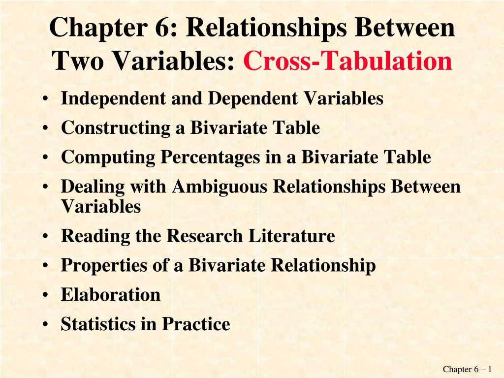
1. Chapter 6: Relationships Between Two Variables: Cross-Tabulation • Independent and Dependent Variables • Constructing a Bivariate Table • Computing Percentages in a Bivariate Table • Dealing with Ambiguous Relationships Between Variables • Reading the Research Literature • Properties of a Bivariate Relationship • Elaboration • Statistics in Practice

2. Introduction • Bivariate Analysis: A statistical method designed to detect and describe the relationship between two variables. • Cross-Tabulation: A technique for analyzing the relationship between two variables that have been organized in a table.

3. Relationship: • As childrenage, theirweightincreases • Largercitieshavemorecrimethansmallercities. • Environmentalconcern, willingnesstotake a cut • Figure 6.1

4. College students who have a history of earning good grades are less likely to miss classes than students who do not. • Contrary to the stereotypes, whites use government safety net programs more than blacks or Latinos, and are more likely to be lifted out of poverty by the taxpayer money they get. • On average, blacks and Latinos have a lower likelihood of access to healthcare than whites.

5. Cross-tabulation • A technique for analyzing the relationship between two variables that have been organized in a table. • Demonstrates not only how to detect whether two variables are associated, but also how to determine the strength of the association and, when appropriate, its direction.

6. Understanding Independent and Dependent Variables • Example: If we hypothesize that English proficiency varies by whether person is native born or foreign born, what is the independent variable, and what is the dependent variable? • Independent: nativity • Dependent: English proficiency

7. Constructing a Bivariate Table • Bivariate table: A table that displays the distribution of one variable across the categories of another variable. • Column variable: A variable whose categories are the columns of a bivariate table. • Row variable:A variable whose categories are the rows of a bivariate table. • Cell: The intersection of a row and a column in a bivariate table. • Marginals: The row and column totals in a bivariate table.

8. Race and homeownership • Table 6.1 • Table 6.2

11. Percentages Can Be Computed in Different Ways: • Column Percentages: column totals as base • Row Percentages: row totals as base

12. Calculate percentages within each category of the independent variable. • When independent variable is arrayed in the columns, compute percentages within each column separately. • Column totals should sum to 100 percent.

13. Race and home ownership • Independent variable: Race • Dependent variable: Home ownership

15. There is a 22.3 percentage point difference between the percentage of white homeowners (55.6%) versus black homeowners (33.3%). • Whites are more likely to be homeowners than blacks. • Race appears to be associated with the likelihood of being a homeowner.

16. Ambiguous relationships between variables • Attitude towards abortion and job security. • Job find: About how easy would it be for you to find a job with another employer with approximately the same income and fringe benefits you now have? (GSS) • Attitude toward abortion: approval or disapproval.

17. Absolute Frequencies Support for Abortion by Job Security Abortion Job Find Easy Job Find Not Easy Row Total Yes 733 40 No 26 23 49 Column Total 33 5689

18. Column Percentages Support for Abortion by Job Security Abortion Job Find Easy Job Find Not Easy Row Total Yes 21% 59% 45% No 79% 41% 55% Column Total 100% 100% 100% (33) (56) (89)

19. Those who feel less secure economically (59%) are more likely to support the right to abortion than those who feel more secure economically (21%). • Hypothesis: Job security is associated with support for abortion. • IV: job security • DV: attitude towards abortion

20. Row Percentages Support for Abortion by Job Security Abortion Job Find Easy Job Find Not Easy Row Total Yes 18% 82% 100% (40) No 53% 47% 100% (49) Column Total 37% 63% 100% (89)

21. Individuals who support abortion are less likely to feel economically secure than those who are against abortion (18% compared with 53%). • Hypothesis: Attitudes toward abortion may be related to one’s sense of job security. • IV: attitude towards abortion • DV: job security

22. Figure 6.2 • What is thetheoreticalquestionposedbytheresearcher? • Not all data can be interpretedusingbothcolumnandrowpercentages. • Genderandattitudetowardsexualharrasment.

23. Medicaid use among the elderly • Table 6.5 • Figure 6.3 • Hypothesis: Gender and race are important determinants of Medicaid use (because U.S. Care system stratifies by gender and race by perpetuating, rather than alleviating, inequality created by social and market forces).

24. Identify dependent variable, unit of analysis. • Identify independent variables and categories. • Clarify the structure of the table (rows/columns). • Determine relationships. • Conclusions?

25. Properties of a Bivariate Relationship • Does there appear to be a relationship? • How strong is it? • What is the direction of the relationship?

26. Existence of a Relationship IV:Church Attendance DV: Support for Abortion If the frequency of church attendance wasunrelated to attitudes toward abortion among women, then we would expect to find equal percentages of people who are pro-choice (or anti-choice), regardless of the level of church attendance. Table 6.7

27. Support for abortion and church attendance • Table 6.6 • Hypothetical illustration of no relationship • Table 6.7

28. Determining the Strength of the Relationship • A quick method is to examine the percentage difference across the different categories of the independent variable. • The larger the percentage difference across the categories, the stronger the association. • We rarely see a situation with either a 0 percent or a 100 percent difference.

29. Direction of the Relationship • Positive relationship: A bivariate relationship between two variables measured at the ordinal level or higher in which the variables vary in the same direction. • Negative relationship: A bivariate relationship between two variables measured at the ordinal level or higher in which the variables vary in opposite directions.

30. A Positive Relationship

31. A Negative Relationship

32. Elaboration • Elaborationis a process designed to further explore a bivariate relationship; it involves the introduction of control variables. • A control variable is an additional variable considered in a bivariate relationship. The variable is controlled for when we take into account its effect on the variables in the bivariate relationship.

33. Three Goals of Elaboration • Elaboration allows us to test for non-spuriousness(that the association cannot be explained away by other variables). • Elaboration clarifies the causal sequence of bivariate relationships by introducing variables hypothesized to intervene between the IV and DV. • Elaboration specifies the different conditions under which the original bivariate relationship might hold.

34. Testing for Nonspuriousness • Direct causal relationship: a bivariate relationship that cannot be accounted for by other theoretically relevant and causally prior variables. • Spurious relationship: a relationship in which both the IV and DV are influenced by a causally prior control variable and there is no causal link between them. The relationship between the IV and DV is said to be “explained away” by the control variable.

35. The Bivariate Relationship Between Number of Firefighters and Property Damage Number of Firefighters  Property Damage (IV) (DV)

37. Process of Elaboration • Partial tables: bivariate tables that display the relationship between the IV and DV while controlling for a third variable. • Partial relationship: the relationship between the IV and DV shown in a partial table.

38. The Process of Elaboration • Divide the observations into subgroups on the basis of the control variable. We have as many subgroups as there are categories in the control variable. • Re-examine the relationship between the original two variables separately for the control variable subgroups. • Compare the partial relationships with the original bivariate relationship for the total group.

41. Intervening Relationship • Intervening variable: a control variable that follows an independent variable but precedes the dependent variable in a causal sequence. • Intervening relationship: a relationship in which the control variable intervenes between the independent and dependent variables.

42. Intervening Relationship:Example Religion  Preferred Family Size  Support for Abortion (IV)(Intervening Control Variable) (DV) • Table 6.10, 6.11, 6.12 • Figure 6.7, 6.8, 6.9

43. Spurious vs. intervening • No causal link – indirect causal link • Causally prior control var – control var follow IV but precedes DV

44. Conditional Relationships • Conditional relationship: a relationship in which the control variable’s effect on the dependent variable is conditional on its interaction with the independent variable. The relationship between the independent and dependent variables will change according to the different conditions of the control variable.

45. Conditional Relationships • Another way to describe a conditional relationship is to say that there is a statistical interaction between the control variable and the independent variable.

46. Conditional Relationships

47. Conditional Relationships

48. Conditional Relationships